1. 背景:相関係数だけでは何が足りないか
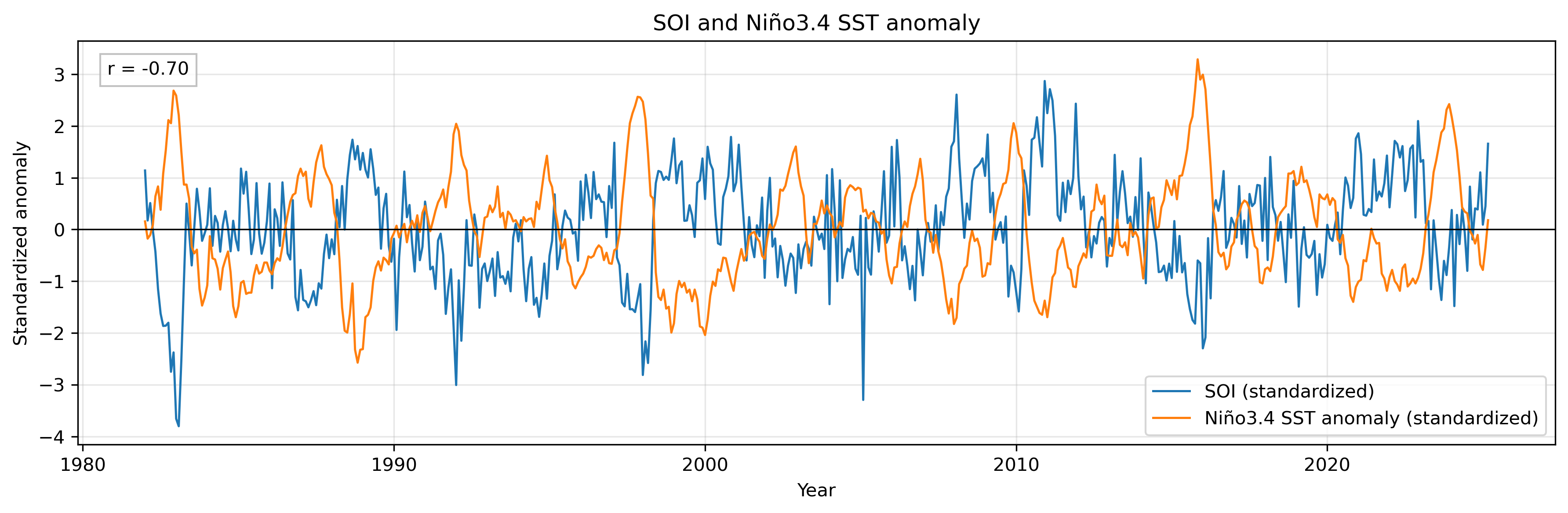
前回までに、SOI と Niño3.4 SST anomaly の相関係数を調べた。今回のデータでは、両者の相関はおよそ r = -0.70 であり、かなり強い負の相関を示す。
しかし、相関係数は時系列全体の関係を1つの数字で表しているだけである。SOI と Niño3.4 の関係が、1年以下の短周期で強いのか、ENSOに対応する2〜7年周期で強いのか、それとももっと長い周期で強いのかは、相関係数だけではわからない。
2. クロススペクトル・コヒーレンス・位相差とは何か
パワースペクトル
パワースペクトルは、1つの時系列にどの周期の変動が強く含まれているかを調べる方法である。
SOI のパワースペクトルなら「SOIの中で何年周期の変動が強いか」、Niño3.4 のパワースペクトルなら「Niño3.4 の中で何年周期の変動が強いか」を見る。
クロススペクトル
クロススペクトルは、2つの時系列がどの周期で共通して変動しているかを調べる方法である。
SOI と Niño3.4 のクロススペクトルが 3〜5年周期で大きければ、両者はその周期帯で共通した変動を持つと考えられる。
コヒーレンス
コヒーレンスは、周期ごとの関係の強さを 0〜1 の値で表す。
- 0に近い:その周期では、2つの時系列はあまり関係していない
- 1に近い:その周期では、2つの時系列は強く関係している
学生向けには、コヒーレンスを「周期ごとの相関係数のようなもの」と説明してよい。ただし、厳密には相関係数そのものではなく、周波数領域で定義される関係の強さである。
位相差
位相差は、ある周期の変動について、2つの時系列が同じタイミングで変動しているのか、片方が先行しているのか、反対向きに変動しているのかを示す。
3. 具体的な計算方法:何を掛け算しているのか
ここがこのページの中心である。クロススペクトル、コヒーレンス、位相差は、いずれも 2つの時系列をフーリエ変換したあとで計算する量である。
ここでは、SOI を x、Niño3.4 SST anomaly を y とする。どちらも平均を引き、標準偏差で割った標準化時系列として扱う。
3.1 まず、2つの時系列をフーリエ変換する
時系列 x と y を、それぞれ周波数成分に分解する。
y(t) → Y(f)
X(f) と Y(f) は、各周波数における複素数である。複素数なので、振幅だけでなく、位相、つまり波のずれの情報も持っている。
3.2 パワースペクトルの計算
パワースペクトルは、各周波数におけるフーリエ成分の大きさの2乗である。
Pyy(f) = |Y(f)|2
Pythonでは、この部分を signal.welch が計算している。
f, Pxx = signal.welch(x, fs=fs, nperseg=nperseg, noverlap=noverlap)
f, Pyy = signal.welch(y, fs=fs, nperseg=nperseg, noverlap=noverlap)
Pxx は SOI のパワースペクトル、Pyy は Niño3.4 SST anomaly のパワースペクトルである。
3.3 クロススペクトルの計算
クロススペクトルは、2つのフーリエ成分を掛け合わせて計算する。考え方としては、片方の複素共役を取り、もう片方と掛ける。
ここで X* は X の複素共役である。SciPy の signal.csd(x, y) も、この考え方でクロススペクトル密度を計算する。
f, Pxy = signal.csd(x, y, fs=fs, nperseg=nperseg, noverlap=noverlap)Pxy は複素数である。そのため、次の2つの情報を含んでいる。
大きさ
np.abs(Pxy)
2つの時系列が、その周期でどれくらい共通して強く変動しているか。
角度
np.angle(Pxy)
2つの時系列が、その周期でどれくらい位相的にずれているか。
このページのクロススペクトル図では、複素数そのものではなく、絶対値を描いている。
cross_power = np.abs(Pxy2)3.4 コヒーレンスの計算
コヒーレンスは、クロススペクトルの大きさを、それぞれのパワースペクトルで規格化した量である。
つまり、クロススペクトルが大きくても、そもそも片方または両方のパワーが非常に大きいだけなら、関係が強いとは限らない。そこで、Pxx と Pyy で割って、0〜1の範囲に正規化する。
Pythonでは signal.coherence がこの計算を行う。
f, coh = signal.coherence(x, y, fs=fs, nperseg=nperseg, noverlap=noverlap)手で書くと、概念的には次の計算である。
coh_manual = np.abs(Pxy)**2 / (Pxx * Pyy)3.5 位相差の計算
位相差は、クロススペクトル Pxy の偏角、つまり複素数の角度として計算する。
Pythonでは次のように計算する。
phase_rad = np.angle(Pxy2)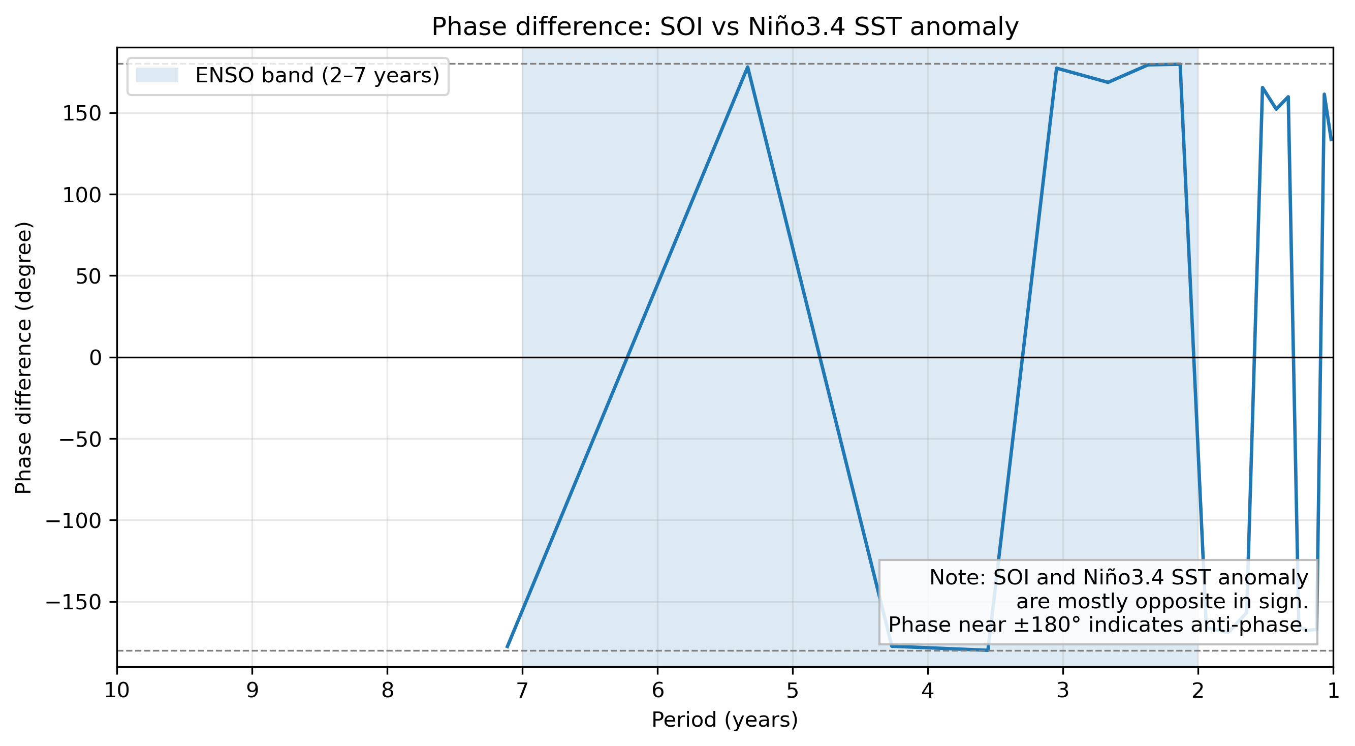
phase_deg = np.degrees(phase_rad)| 位相差 | 読み方 |
|---|---|
| 0°付近 | 同じ周期で、ほぼ同じタイミング・同じ向きに変動している。 |
| +90° または −90°付近 | 片方が約1/4周期だけ先行・遅延している。 |
| ±180°付近 | 同じ周期で、ほぼ反対向きに変動している。 |
SOI と Niño3.4 SST anomaly は符号が逆になりやすいので、ENSO周期帯では ±180°付近に出やすい。この場合は「大きなラグがある」ではなく、「反位相である」と読む。
3.6 位相差からラグへ換算する
位相差を時間のずれに換算することもできる。周波数を f、位相差をラジアンで phase_rad とすると、
このページでは周波数の単位が cycles/year なので、まず年単位のラグが得られ、それを12倍して月に変換している。
lag_year = phase_rad / (2.0 * np.pi * f2)
lag_month = lag_year * 12.03.7 Welch法で平均している理由
1回だけFFTをかけると、スペクトルはかなりギザギザになりやすい。Welch法では、時系列をいくつかの短い区間に分け、それぞれに窓関数をかけてスペクトルを計算し、最後に平均する。
今回の nperseg = 256 は、1区間を256か月、つまり約21.3年にするという意味である。noverlap = 128 なので、隣の区間とは半分重ねて計算している。
4. 使用データ
使用するデータは、前回までと同じである。HTML と同じディレクトリに次のファイルを置く。
| ファイル | 使う列 | 内容 |
|---|---|---|
| sstoi.indices | ANOM34 | Niño3.4 領域の海面水温偏差 |
| SOI_timeseries_updated.txt | SOI | 南方振動指数 |
5. 計算の流れ
- SOI と Niño3.4 SST anomaly を読み込む
- YEAR と MONTH で結合し、共通期間だけを使う
- 平均を引き、標準偏差で割って標準化する
- Welch法でそれぞれのパワースペクトルを計算する
- signal.csd でクロススペクトルを計算する
- signal.coherence でコヒーレンスを計算する
- 周波数を周期に変換し、2〜7年のENSO帯に注目する
- 位相差を計算し、反位相かどうかを確認する
6. クロススペクトル・コヒーレンスのPythonスクリプト
以下は、Jupyter Lab の1セルに貼って実行できる完全スクリプトである。図は PNG と PDF の両方で保存される。
完全スクリプトを表示
import os
import numpy as np
import pandas as pd
import matplotlib.pyplot as plt
from scipy import signal

# ============================================================
# 0. 設定
# ============================================================
soi_file = "SOI_timeseries_updated.txt"
sst_file = "sstoi.indices"

outdir = "fig_cross_spectrum_soi_nino34"
os.makedirs(outdir, exist_ok=True)

# 月平均データなので、1年あたり12点
fs = 12

# Welch法の窓長
# 256か月 = 約21.3年
nperseg = 256
noverlap = nperseg // 2

# 表示する周期範囲
period_min = 1.0
period_max = 10.0

# ENSO周期帯
enso_min = 2.0
enso_max = 7.0


def savefig(fig, filename_base):
    png_path = os.path.join(outdir, filename_base + ".png")
    pdf_path = os.path.join(outdir, filename_base + ".pdf")
    fig.tight_layout()
    fig.savefig(png_path, dpi=300, bbox_inches="tight")
    fig.savefig(pdf_path, bbox_inches="tight")
    print("Saved:", png_path)
    print("Saved:", pdf_path)
    plt.show()


# ============================================================
# 1. データ読み込み
# ============================================================
soi = pd.read_csv(soi_file, sep=r"\s+")

cols = [
    "YEAR", "MONTH",
    "NINO12", "ANOM12",
    "NINO3",  "ANOM3",
    "NINO4",  "ANOM4",
    "NINO34", "ANOM34"
]

sst = pd.read_csv(
    sst_file,
    sep=r"\s+",
    skiprows=1,
    names=cols
)

for c in cols:
    sst[c] = pd.to_numeric(sst[c], errors="coerce")

for c in ["YEAR", "MONTH", "SOI", "TIME"]:
    soi[c] = pd.to_numeric(soi[c], errors="coerce")


# ============================================================
# 2. 年月で結合
# ============================================================
df = pd.merge(
    soi,
    sst,
    on=["YEAR", "MONTH"],
    how="inner"
)

df = df.dropna(subset=["SOI", "ANOM34", "TIME"]).reset_index(drop=True)

print("Number of months =", len(df))
print("Start:", int(df["YEAR"].iloc[0]), int(df["MONTH"].iloc[0]))
print("End  :", int(df["YEAR"].iloc[-1]), int(df["MONTH"].iloc[-1]))

if len(df) < nperseg:
    raise ValueError("Data length is shorter than nperseg. Use smaller nperseg, e.g. 128.")


# ============================================================
# 3. 解析に使う時系列
# ============================================================
time = df["TIME"].to_numpy()
x_raw = df["SOI"].to_numpy()
y_raw = df["ANOM34"].to_numpy()

# 平均を引く
x = x_raw - np.nanmean(x_raw)
y = y_raw - np.nanmean(y_raw)

# 標準化
x = x / np.nanstd(x)
y = y / np.nanstd(y)

good = np.isfinite(x) & np.isfinite(y) & np.isfinite(time)
x = x[good]
y = y[good]
time = time[good]

r0 = np.corrcoef(x, y)[0, 1]
print("Correlation between SOI and Niño3.4 SST anomaly =", r0)


# ============================================================
# 4. パワースペクトル、クロススペクトル、コヒーレンス
# ============================================================
f, Pxx = signal.welch(
    x, fs=fs, window="hann",
    nperseg=nperseg, noverlap=noverlap,
    detrend="constant", scaling="density"
)

f, Pyy = signal.welch(
    y, fs=fs, window="hann",
    nperseg=nperseg, noverlap=noverlap,
    detrend="constant", scaling="density"
)

# クロススペクトル:Pxy は複素数
f, Pxy = signal.csd(
    x, y, fs=fs, window="hann",
    nperseg=nperseg, noverlap=noverlap,
    detrend="constant", scaling="density"
)

# コヒーレンス
f, coh = signal.coherence(
    x, y, fs=fs, window="hann",
    nperseg=nperseg, noverlap=noverlap,
    detrend="constant"
)

valid = f > 0
f2 = f[valid]
period = 1.0 / f2

Pxx2 = Pxx[valid]
Pyy2 = Pyy[valid]
Pxy2 = Pxy[valid]
coh2 = coh[valid]

cross_power = np.abs(Pxy2)
phase_rad = np.angle(Pxy2)
phase_deg = np.degrees(phase_rad)

phase_unwrap_rad = np.unwrap(phase_rad)
phase_unwrap_deg = np.degrees(phase_unwrap_rad)

lag_year = phase_rad / (2.0 * np.pi * f2)
lag_month = lag_year * 12.0

m = (period >= period_min) & (period <= period_max)
period_plot = period[m]
Pxx_plot = Pxx2[m]
Pyy_plot = Pyy2[m]
cross_plot = cross_power[m]
coh_plot = coh2[m]
phase_plot = phase_deg[m]
phase_unwrap_plot = phase_unwrap_deg[m]
lag_plot = lag_month[m]

enso_band_all = (period >= enso_min) & (period <= enso_max)
mean_coh_enso = np.nanmean(coh2[enso_band_all])
max_coh_enso = np.nanmax(coh2[enso_band_all])
period_max_coh = period[enso_band_all][np.nanargmax(coh2[enso_band_all])]

print(f"Mean coherence in ENSO band ({enso_min:g}–{enso_max:g} years): {mean_coh_enso:.3f}")
print(f"Max coherence in ENSO band ({enso_min:g}–{enso_max:g} years): {max_coh_enso:.3f}")
print(f"Period of max coherence in ENSO band: {period_max_coh:.2f} years")


# ============================================================
# 5. 図1:時系列
# ============================================================
fig, ax = plt.subplots(figsize=(12, 4))
ax.plot(time, x, label="SOI (standardized)", linewidth=1.2)
ax.plot(time, y, label="Niño3.4 SST anomaly (standardized)", linewidth=1.2)
ax.axhline(0, color="k", linewidth=0.8)
ax.set_xlabel("Year")
ax.set_ylabel("Standardized anomaly")
ax.set_title("SOI and Niño3.4 SST anomaly")
ax.legend(loc="lower right")
ax.grid(True, alpha=0.3)
ax.text(0.02, 0.95, f"r = {r0:.2f}", transform=ax.transAxes,
        va="top", ha="left",
        bbox=dict(facecolor="white", edgecolor="0.7", alpha=0.8))
savefig(fig, "fig01_timeseries_soi_nino34")


# ============================================================
# 6. 図2:パワースペクトル
# ============================================================
fig, ax = plt.subplots(figsize=(9, 5))
ax.plot(period_plot, Pxx_plot, label="SOI", linewidth=1.8)
ax.plot(period_plot, Pyy_plot, label="Niño3.4 SST anomaly", linewidth=1.8)
ax.axvspan(enso_min, enso_max, alpha=0.15, label="ENSO band (2–7 years)")
ax.set_xlabel("Period (years)")
ax.set_ylabel("Power spectral density")
ax.set_title("Power spectra")
ax.set_xlim(period_max, period_min)
ax.legend(loc="upper left")
ax.grid(True, alpha=0.3)
savefig(fig, "fig02_power_spectra")


# ============================================================
# 7. 図3:クロススペクトル
# ============================================================
fig, ax = plt.subplots(figsize=(9, 5))
ax.plot(period_plot, cross_plot, linewidth=1.8)
ax.axvspan(enso_min, enso_max, alpha=0.15, label="ENSO band (2–7 years)")
ax.set_xlabel("Period (years)")
ax.set_ylabel("|Cross spectrum|")
ax.set_title("Cross spectrum: SOI vs Niño3.4 SST anomaly")
ax.set_xlim(period_max, period_min)
ax.legend(loc="upper left")
ax.grid(True, alpha=0.3)
savefig(fig, "fig03_cross_spectrum")


# ============================================================
# 8. 図4:コヒーレンス
# ============================================================
fig, ax = plt.subplots(figsize=(9, 5))
ax.plot(period_plot, coh_plot, linewidth=1.8)
ax.axvspan(enso_min, enso_max, alpha=0.15, label="ENSO band (2–7 years)")
ax.set_xlabel("Period (years)")
ax.set_ylabel("Coherence")
ax.set_title("Coherence: SOI vs Niño3.4 SST anomaly")
ax.set_xlim(period_max, period_min)
ax.set_ylim(0, 1.05)
ax.legend(loc="upper left")
ax.grid(True, alpha=0.3)
text = (f"Mean coherence ({enso_min:g}–{enso_max:g} yr) = {mean_coh_enso:.2f}\n"
        f"Max coherence = {max_coh_enso:.2f}\n"
        f"Peak period = {period_max_coh:.2f} yr")
ax.text(0.98, 0.05, text, transform=ax.transAxes,
        va="bottom", ha="right",
        bbox=dict(facecolor="white", edgecolor="0.7", alpha=0.85))
savefig(fig, "fig04_coherence")


# ============================================================
# 9. 図5:位相差
# ============================================================
fig, ax = plt.subplots(figsize=(9, 5))
ax.plot(period_plot, phase_plot, linewidth=1.6)
ax.axhline(0, color="k", linewidth=0.8)
ax.axhline(180, color="gray", linestyle="--", linewidth=0.8)
ax.axhline(-180, color="gray", linestyle="--", linewidth=0.8)
ax.axvspan(enso_min, enso_max, alpha=0.15, label="ENSO band (2–7 years)")
ax.set_xlabel("Period (years)")
ax.set_ylabel("Phase difference (degree)")
ax.set_title("Phase difference: SOI vs Niño3.4 SST anomaly")
ax.set_xlim(period_max, period_min)
ax.set_ylim(-190, 190)
ax.legend(loc="upper left")
ax.grid(True, alpha=0.3)
ax.text(0.98, 0.05,
        "Note: SOI and Niño3.4 SST anomaly\nare mostly opposite in sign.\nPhase near ±180° indicates anti-phase.",
        transform=ax.transAxes, va="bottom", ha="right",
        bbox=dict(facecolor="white", edgecolor="0.7", alpha=0.85))
savefig(fig, "fig05_phase_raw")


# ============================================================
# 10. 図6:まとめ図
# ============================================================
fig, axes = plt.subplots(3, 1, figsize=(10, 12), sharex=False)

axes[0].plot(period_plot, Pxx_plot, label="SOI", linewidth=1.6)
axes[0].plot(period_plot, Pyy_plot, label="Niño3.4 SST anomaly", linewidth=1.6)
axes[0].axvspan(enso_min, enso_max, alpha=0.15)
axes[0].set_ylabel("Power spectral density")
axes[0].set_title("Power spectra")
axes[0].set_xlim(period_max, period_min)
axes[0].legend(loc="upper left")
axes[0].grid(True, alpha=0.3)

axes[1].plot(period_plot, cross_plot, linewidth=1.6)
axes[1].axvspan(enso_min, enso_max, alpha=0.15)
axes[1].set_ylabel("|Cross spectrum|")
axes[1].set_title("Cross spectrum")
axes[1].set_xlim(period_max, period_min)
axes[1].grid(True, alpha=0.3)

axes[2].plot(period_plot, coh_plot, linewidth=1.8)
axes[2].axvspan(enso_min, enso_max, alpha=0.15, label="ENSO band (2–7 years)")
axes[2].set_xlabel("Period (years)")
axes[2].set_ylabel("Coherence")
axes[2].set_title("Coherence")
axes[2].set_xlim(period_max, period_min)
axes[2].set_ylim(0, 1.05)
axes[2].legend(loc="upper left")
axes[2].grid(True, alpha=0.3)
axes[2].text(0.98, 0.05,
             f"Mean coherence = {mean_coh_enso:.2f}\nMax coherence = {max_coh_enso:.2f}\nPeak = {period_max_coh:.2f} yr",
             transform=axes[2].transAxes,
             va="bottom", ha="right",
             bbox=dict(facecolor="white", edgecolor="0.7", alpha=0.85))
savefig(fig, "fig08_summary_power_cross_coherence")
スクリプトの逐一説明
| コード | 意味 |
|---|---|
| fs = 12 | 月平均データなので、1年に12個のデータがあるという意味。 |
| nperseg = 256 | Welch法で1回に使うデータ長。256か月、つまり約21年の窓でスペクトルを計算する。 |
| signal.welch | 1つの時系列のパワースペクトルを計算する。 |
| signal.csd | 2つの時系列のクロススペクトルを計算する。結果は複素数になる。 |
| signal.coherence | 周期ごとの関係の強さを0〜1で計算する。 |
| period = 1.0 / f2 | 周波数を周期に変換する。単位は年。 |
| np.abs(Pxy2) | クロススペクトルの大きさを取り出す。 |
| np.angle(Pxy2) | クロススペクトルの角度、つまり位相差を取り出す。 |
| np.abs(Pxy2)**2 / (Pxx2 * Pyy2) | コヒーレンスの定義。実際の計算は signal.coherence が行う。 |
| phase_rad / (2*np.pi*f2) | 位相差を時間ラグに換算する式。ただし反位相の場合は解釈に注意する。 |
7. 図の読み方
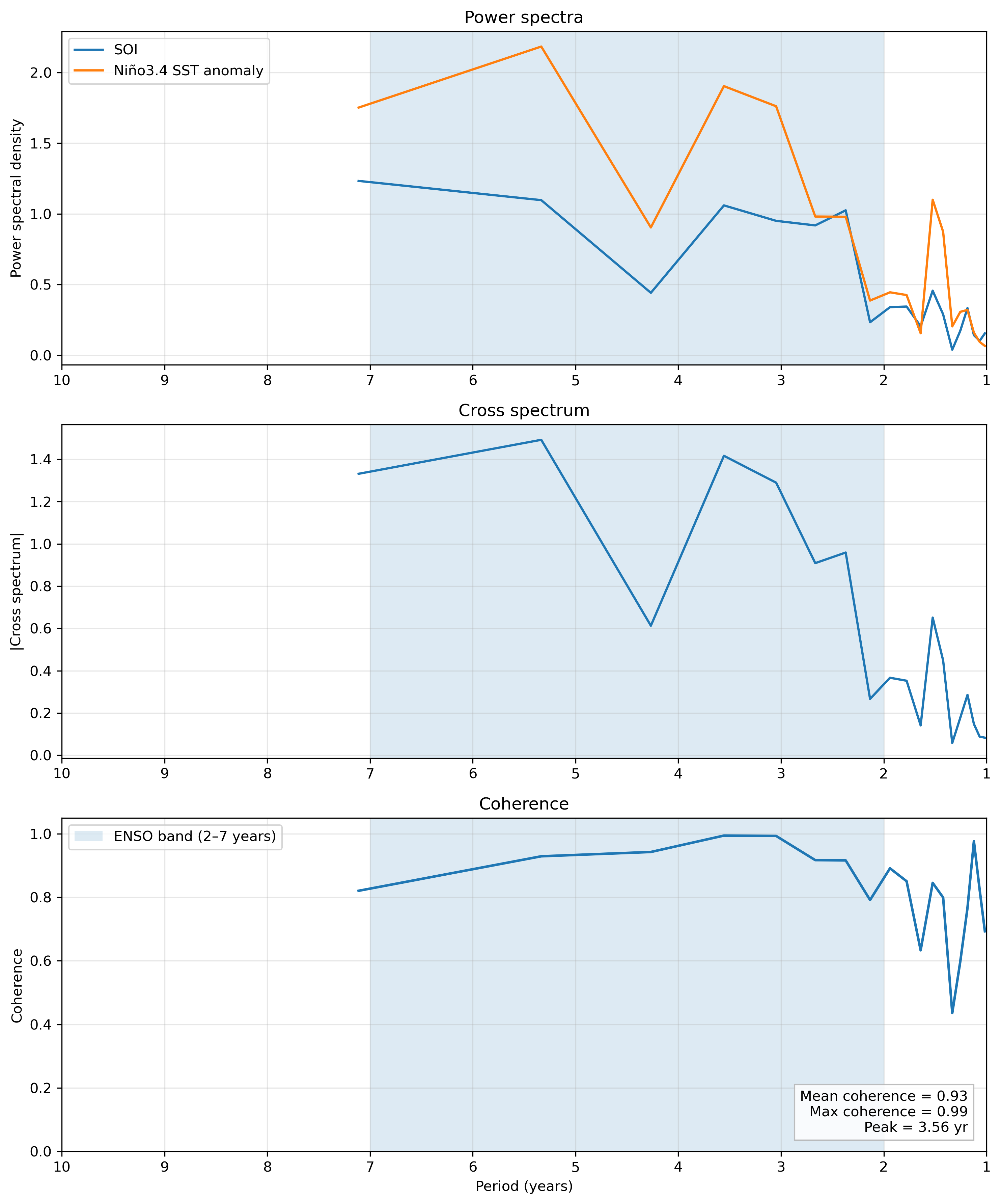
上段:パワースペクトル
SOI と Niño3.4 SST anomaly が、それぞれどの周期帯に強い変動を持つかを見る。2〜7年帯にパワーがあるなら、ENSOに関連する周期変動が含まれていると考えられる。
中段:クロススペクトル
2つの時系列に共通する周期変動の強さを見る。3〜6年付近で大きければ、SOI と Niño3.4 はENSO周期帯で共通した変動を持つと読める。
下段:コヒーレンス
今回の結果では、2〜7年周期帯でコヒーレンスが高く、平均値は約0.93、最大値は約0.99である。これは、SOI と Niño3.4 SST anomaly がENSO周期帯で非常に強く結びついていることを示す。
8. 位相差とラグの注意点
位相差は重要だが、読み方を間違えやすい。特に SOI と Niño3.4 SST anomaly は符号が逆に変動しやすいため、位相差は180°付近に現れやすい。
9. 補足:Wavelet解析とは何か
ここまでのスペクトル解析では、全期間をまとめて「どの周期が強いか」を見た。しかし ENSO の強さは時代によって変わる。1980年代、1997–1998年、2015–2016年など、強いEl Niñoが発生した時期とそうでない時期がある。
Wavelet解析は、時間方向と周期方向を同時に見る方法である。
| 軸 | 意味 |
|---|---|
| 横軸 | 時間 |
| 縦軸 | 周期 |
| 色 | その時期・その周期における変動の強さ |
| COI | 端の影響を受けやすい領域の目安 |
10. Wavelet解析のPythonスクリプト
Wavelet は難しいので、ここでは穴埋めにせず、完全スクリプトとして示す。Jupyter Lab で実行する場合、PyWavelets が入っていなければ、事前に pip install PyWavelets を実行する。
Wavelet完全スクリプトを表示
import numpy as np
import pandas as pd
import matplotlib.pyplot as plt
import pywt

# =========================================================
# 0. 設定
# =========================================================
soi_file = "SOI_timeseries_updated.txt"
nino_file = "sstoi.indices"

fig_nino_name = "wavelet_nino34_improved.png"
fig_soi_name  = "wavelet_soi_improved.png"

# 月平均データ:dt は年単位
# 1か月 = 1/12年
dt_year = 1.0 / 12.0

# モール波
wavelet_name = "morl"

# スケール範囲
# 大きくすると長周期まで見ることができる
scales = np.arange(1, 256)

# ENSO帯(年)
enso_min_year = 2.0
enso_max_year = 7.0


# =========================================================
# 1. データ読み込み
# =========================================================
colnames = [
    "YR", "MON",
    "NINO12", "ANOM12",
    "NINO3",  "ANOM3",
    "NINO4",  "ANOM4",
    "NINO34", "ANOM34"
]

nino_df = pd.read_csv(
    nino_file,
    sep=r"\s+",
    skiprows=1,
    names=colnames
)

nino_time = nino_df["YR"].values + (nino_df["MON"].values - 1) / 12.0
nino_x = nino_df["ANOM34"].values.astype(float)

soi_df = pd.read_csv(soi_file, sep=r"\s+")
soi_time = soi_df["TIME"].values
soi_x = soi_df["SOI"].values.astype(float)


# =========================================================
# 2. 前処理関数
# =========================================================
def standardize(x):
    x = np.asarray(x, dtype=float)
    if np.any(~np.isfinite(x)):
        x = pd.Series(x).interpolate(limit_direction="both").values
    x = x - np.mean(x)
    x = x / np.std(x)
    return x


# =========================================================
# 3. Wavelet図作成関数
# =========================================================
def wavelet_plot_with_coi(x, time, title, ylabel, save_name,
                          wavelet_name="morl", scales=None,
                          enso_min_year=2.0, enso_max_year=7.0):
    x = standardize(x)

    coef, freqs = pywt.cwt(
        x,
        scales,
        wavelet_name,
        sampling_period=dt_year
    )

    power = np.abs(coef) ** 2

    # 周期(年)
    period_year = 1.0 / freqs

    # COIの簡易的な目安
    # 端に近いほど長周期成分は信頼しにくい
    n = len(x)
    edge_dist = np.minimum(np.arange(n), np.arange(n)[::-1])
    coi = np.sqrt(2) * edge_dist * dt_year

    fig, ax = plt.subplots(figsize=(14, 7))

    levels = np.linspace(0, np.nanpercentile(power, 99), 20)
    cf = ax.contourf(time, period_year, power, levels=levels, cmap="RdBu_r", extend="max")

    # ENSO帯を線で示す
    ax.axhline(enso_min_year, color="k", linestyle="--", linewidth=1.0)
    ax.axhline(enso_max_year, color="k", linestyle="--", linewidth=1.0)
    ax.text(time[0] + 0.02 * (time[-1] - time[0]),
            (enso_min_year + enso_max_year) / 2,
            "ENSO band (2–7 years)",
            va="center", ha="left",
            bbox=dict(facecolor="white", edgecolor="none", alpha=0.8))

    # COIを描く
    ax.plot(time, coi, color="gray", linewidth=1.5, label="COI")
    ax.fill_between(time, coi, period_year.max(), color="gray", alpha=0.25)

    ax.set_yscale("log")
    ax.set_ylim(period_year.max(), period_year.min())
    ax.set_ylabel(ylabel)
    ax.set_xlabel("Time")
    ax.set_title(title, fontsize=16)
    ax.grid(True, alpha=0.25)
    ax.legend(loc="upper right")

    cbar = fig.colorbar(cf, ax=ax, pad=0.02)
    cbar.set_label("Power")

    fig.savefig(save_name, dpi=300, bbox_inches="tight", facecolor="white")
    plt.show()
    print(f"Saved: {save_name}")


# =========================================================
# 4. 実行
# =========================================================
wavelet_plot_with_coi(
    x=nino_x,
    time=nino_time,
    title="Wavelet Power Spectrum (Niño3.4)",
    ylabel="Period (years)",
    save_name=fig_nino_name,
    wavelet_name=wavelet_name,
    scales=scales,
    enso_min_year=enso_min_year,
    enso_max_year=enso_max_year
)

wavelet_plot_with_coi(
    x=soi_x,
    time=soi_time,
    title="Wavelet Power Spectrum (SOI)",
    ylabel="Period (years)",
    save_name=fig_soi_name,
    wavelet_name=wavelet_name,
    scales=scales,
    enso_min_year=enso_min_year,
    enso_max_year=enso_max_year
)
Wavelet図の見方
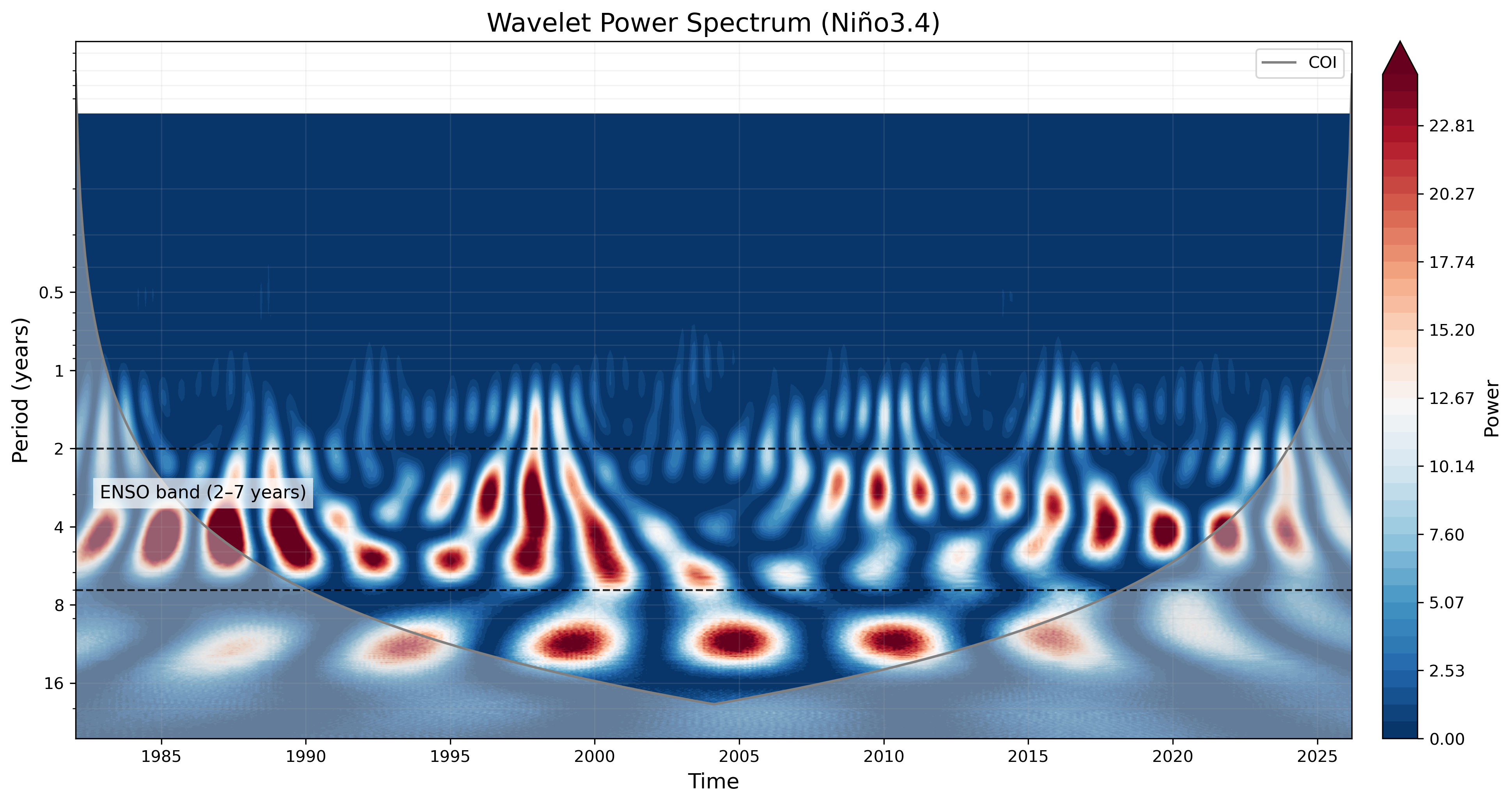
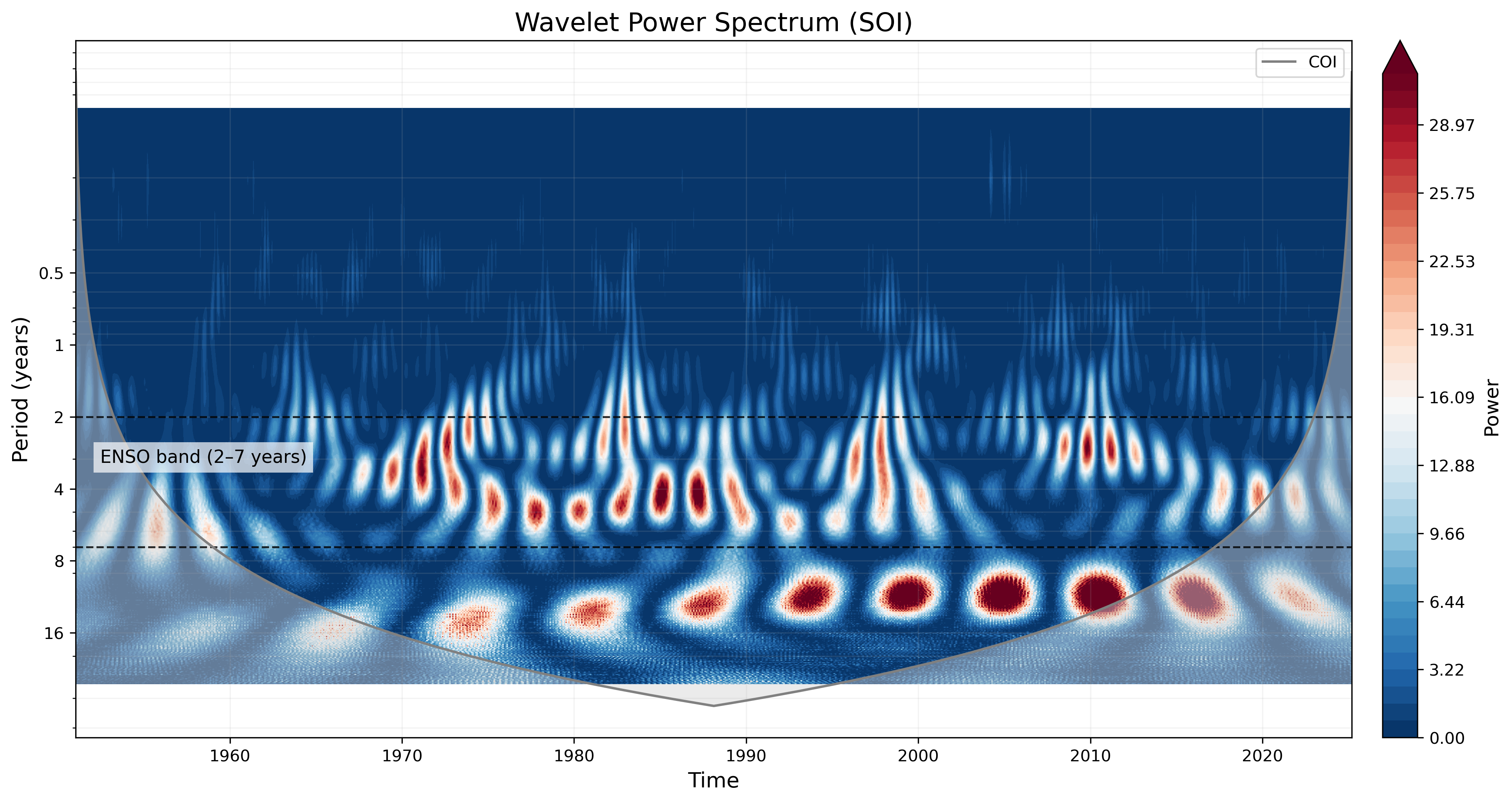
Wavelet図で見ること
- 2〜7年帯に赤い領域があるか
- その赤い領域が、どの時期に強いか
- Niño3.4 と SOI で、ENSO帯の強い時期が対応しているか
- COI の外側・端に近い部分を過度に解釈していないか
11. それぞれ何を見ているのか
| 解析 | 見るもの | この講義での解釈 |
|---|---|---|
| 相関係数 | 全期間をまとめた2時系列の関係 | SOI と Niño3.4 は全体として強い負相関を持つ。 |
| ラグ相関 | 片方をずらしたときの関係 | 明瞭な時間遅れは小さく、ほぼ同時に反対向きに変動する。 |
| パワースペクトル | 1つの時系列の周期成分 | SOI と Niño3.4 の両方に ENSO帯の変動がある。 |
| クロススペクトル | 2時系列に共通する周期成分 | 2〜7年帯、特に3〜6年付近で共通変動が強い。 |
| コヒーレンス | 周期ごとの関係の強さ | ENSO帯で高いので、両者はこの周期帯で強く結びつく。 |
| 位相差 | 周期ごとのずれ・反位相 | ±180°付近は、SOI と Niño3.4 が反位相であることを示す。 |
| Wavelet | いつ・どの周期が強いか | ENSO帯の変動は常に同じ強さではなく、時代によって強弱がある。 |
12. 考える課題
- SOI と Niño3.4 の相関係数は負である。これは物理的に何を意味しているか。
- パワースペクトルとクロススペクトルの違いを、自分の言葉で説明せよ。
- コヒーレンスが 2〜7年周期帯で高いことは、ENSOの理解において何を意味するか。
- 位相差が ±180° 付近にあることを、「時間遅れ」とだけ読んではいけない理由を説明せよ。
- Wavelet図では、ENSO帯の強い変動がいつでも同じように出ているか。Niño3.4 と SOI を比較して述べよ。