1. 背景:コンポジットとは何か
気候・海洋データでは、毎年の値はばらつきが大きい。ある現象が起きたときの典型的な空間パターンを見たい場合には、条件を満たす時期だけを集めて平均する。この条件付き平均を コンポジット という。
La Niña composite SST = La Niña と判定された月の SST の平均
2. 使用データ
ENSO 判定には sstoi.indices、全球 SST には sst.mnmean.nc を使う。HTML と同じディレクトリに置く。
| ファイル | 使う変数・列 | 内容 |
|---|---|---|
| sstoi.indices | ANOM34 | Niño3.4 anomaly |
| sst.mnmean.nc | sst(time, lat, lon) | 全球月平均 SST |
3. ENSO の判定方法
1か月だけ閾値を超えた場合は短期的な揺らぎかもしれない。そこで、3か月移動平均をとったうえで、一定期間以上続いた月だけをイベントとする。
| 現象 | 判定条件 |
|---|---|
| El Niño | 3か月移動平均した Niño3.4 anomaly が +0.5℃以上を 3か月以上継続 |
| La Niña | 3か月移動平均した Niño3.4 anomaly が −0.5℃以下を 3か月以上継続 |
ENSO は数か月以上続く現象なので、月ごとの細かいノイズではなく、継続的な偏差を見る。
4. 計算の流れ
- Niño3.4 anomaly を読み込む
- 3か月移動平均を計算する
- +0.5℃ / −0.5℃ が3か月以上続く月を判定する
- SST データを読み込む
- 年月単位で ENSO 判定を SST に対応付ける
- El Niño, La Niña, 差分のコンポジット図を保存する
5. 設定
使用するファイル名、閾値、保存する図のファイル名を設定する。
import numpy as np
import pandas as pd
import xarray as xr
import matplotlib.pyplot as plt

# =========================================================
# 0. 設定
# =========================================================
sst_file = ______
nino_file = ______

threshold = ______   # Niño3.4 anomaly threshold [degC]
min_len = ______       # minimum duration [months]

# 保存ファイル名
fig_ts_name   = "enso_event_detection.png"
fig_comp_name = "enso_composite_sst.png"
fig_anom_name = "enso_composite_sst_anomaly.png"6. Niño3.4 データの読み込み
sstoi.indices に列名を付け、Niño3.4 anomaly を取り出す。
# =========================================================
# 1. sstoi.indices を読む
#    最後の ANOM が Nino3.4 anomaly
# =========================================================
colnames = [
    "YR", "MON",
    "NINO12", "ANOM12",
    "NINO3",  "ANOM3",
    "NINO4",  "ANOM4",
    "NINO34", "ANOM34"
]

df = pd.read_csv(
    nino_file,
    sep=______,
    skiprows=______,
    names=______
)

# 年月を datetime に
df["time"] = pd.to_datetime(dict(year=df[______], month=df[______], day=15))

# 月キー(YYYY-MM)を作る
df["ym"] = df["time"].dt.to_period(______)

# Niño3.4 anomaly
nino34_anom = pd.Series(df[______].values, index=df["time"])

print("=== sstoi.indices preview ===")
print(df.head())
print()7. 3か月移動平均
月々の細かい揺らぎをならすため、Niño3.4 anomaly に 3か月移動平均をかける。
# =========================================================
# 2. 3か月移動平均
# =========================================================
nino34_smooth = nino34_anom.rolling(window=______, center=True).mean()8. 3か月以上継続するイベント抽出
閾値を超えた状態が何か月続いたかを数え、3か月以上続いた月だけを ENSO イベントとして True にする。
# =========================================================
# 3. 3か月以上継続するイベント抽出
# =========================================================
def detect_runs(series, threshold=0.5, mode=______, min_len=5):
    if mode == "el":
        mask = series ______ threshold
    elif mode == "la":
        mask = series ______ -threshold
    else:
        raise ValueError("mode must be 'el' or 'la'")

    events = np.zeros(len(series), dtype=bool)
    count = 0

    for i in range(len(series)):
        if pd.notna(mask.iloc[i]) and mask.iloc[i]:
            count ______ 1
        else:
            if count >= min_len:
                events[i-count:i] = ______
            count = 0

    if count >= min_len:
        events[len(series)-count:len(series)] = ______

    return pd.Series(events, index=series.index)

el_event = detect_runs(nino34_smooth, threshold=threshold, mode=______, min_len=min_len)
la_event = detect_runs(nino34_smooth, threshold=threshold, mode=______, min_len=min_len)9. イベント年の確認
検出された El Niño / La Niña の年と月数を表示して、イベント判定が極端におかしくないか確認する。
# =========================================================
# 4. イベント年を表示
# =========================================================
el_years = np.unique(el_event.index[______].year)
la_years = np.unique(la_event.index[______].year)

print("=== Event years ===")
print("El Niño years :", el_years)
print("La Niña years :", la_years)
print()

print("El Niño months :", int(el_event.sum()))
print("La Niña months :", int(la_event.sum()))
print()10. ENSO判定図
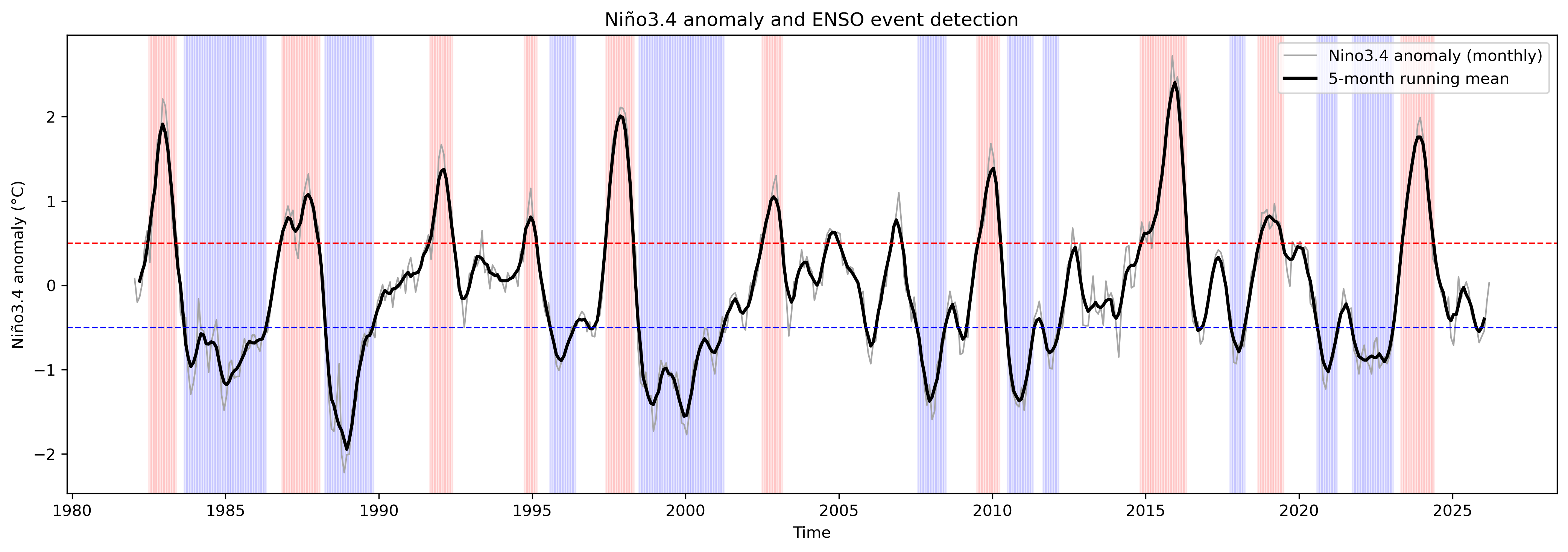
月ごとの Niño3.4 anomaly、3か月移動平均、El Niño / La Niña 判定月を同じ図に描く。
# =========================================================
# 5. ENSO判定図
# =========================================================
plt.figure(figsize=(14, 5))
plt.plot(nino34_anom.index, nino34_anom.values, color="0.65", lw=1.0, label="Nino3.4 anomaly (monthly)")
plt.plot(nino34_smooth.index, nino34_smooth.values, color="k", lw=2.0, label="3-month running mean")

plt.axhline(threshold, color="r", ls="--", lw=1)
plt.axhline(-threshold, color="b", ls="--", lw=1)

for t in el_event.index[el_event]:
    plt.axvspan(t - pd.Timedelta(days=15), t + pd.Timedelta(days=15), color="red", alpha=0.08)

for t in la_event.index[la_event]:
    plt.axvspan(t - pd.Timedelta(days=15), t + pd.Timedelta(days=15), color="blue", alpha=0.08)

plt.title("Niño3.4 anomaly and ENSO event detection")
plt.ylabel("Niño3.4 anomaly (°C)")
plt.xlabel("Time")
plt.legend(loc="upper right")
plt.tight_layout()
plt.savefig(fig_ts_name, dpi=300, bbox_inches="tight", facecolor="white")
plt.show()

print(f"Saved: {fig_ts_name}")11. SST データの読み込み
ERSST の月平均 SST を xarray で読み込み、欠損値を除外する。
# =========================================================
# 6. SST 読み込み
# =========================================================
ds = xr.open_dataset(______)
sst = ds[______].astype(float)

# 欠損値処理
sst = sst.where(sst > ______)

# SSTの時間
time_sst = pd.to_datetime(ds["time"].values)
ym_sst = pd.Series(time_sst).dt.to_period("M")

print("=== SST dataset info ===")
print(ds)
print()12. ENSOイベントを SST に対応付ける
Niño 指数と SST では日付がずれることがあるので、年月 YYYY-MM で対応付ける。
# =========================================================
# 7. 月単位で ENSOイベントを SST に対応付ける
# =========================================================
event_df = pd.DataFrame({
    "ym": df["ym"],
    "el": el_event.values,
    "la": la_event.values
})

# ym ごとに辞書化
el_map = dict(zip(event_df["ym"], event_df[______]))
la_map = dict(zip(event_df["ym"], event_df[______]))

el_mask_sst = np.array([el_map.get(ym, False) for ym in ym_sst], dtype=bool)
la_mask_sst = np.array([la_map.get(ym, False) for ym in ym_sst], dtype=bool)

print("Matched El Niño months in SST :", el_mask_sst.sum())
print("Matched La Niña months in SST :", la_mask_sst.sum())
print()

# 安全確認
if el_mask_sst.sum() == 0:
    raise ValueError("El Niño months matched to SST are zero.")
if la_mask_sst.sum() == 0:
raise ValueError("La Niña months matched to SST are zero.")13. コンポジット平均の計算
El Niño 月、La Niña 月だけを抽出し、それぞれの SST 平均と差分を計算する。
# =========================================================
# 8. コンポジット計算
# =========================================================
sst_el = sst.isel(time=______)
sst_la = sst.isel(time=______)

comp_el = sst_el.mean(dim=______)
comp_la = sst_la.mean(dim=______)
comp_diff = ______ - ______

# 全期間平均
clim_all = sst.mean(dim=______)
comp_el_anom = comp_el - clim_all
comp_la_anom = comp_la - clim_all

# 値の確認
print("comp_el min/max  :", float(comp_el.min()), float(comp_el.max()))
print("comp_la min/max  :", float(comp_la.min()), float(comp_la.max()))
print("comp_diff min/max:", float(comp_diff.min()), float(comp_diff.max()))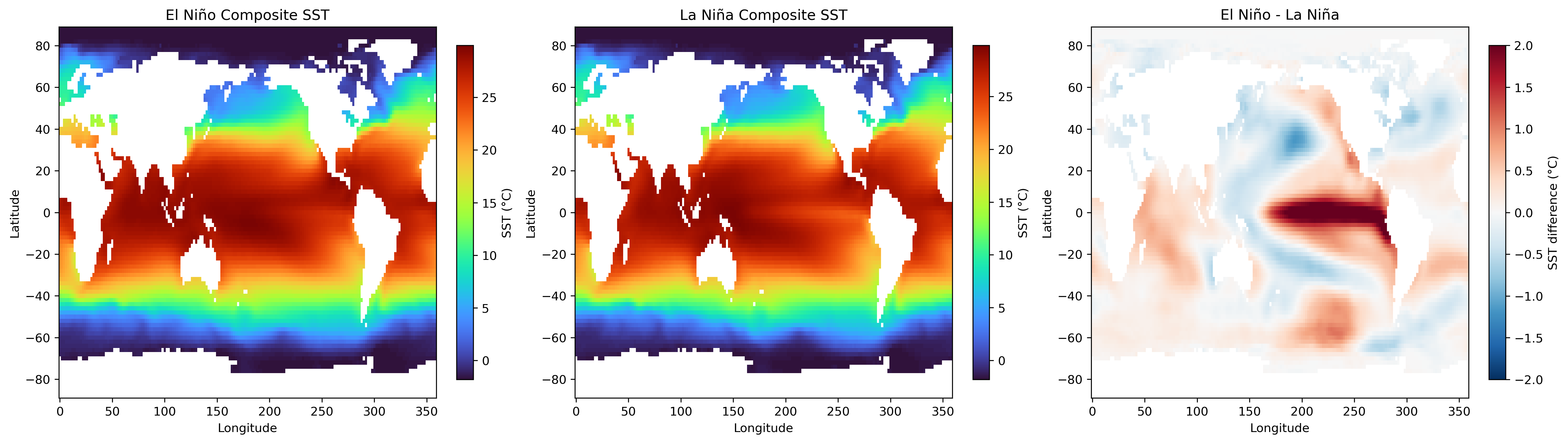
print()14. 絶対値 SST コンポジット図
El Niño composite SST、La Niña composite SST、El Niño − La Niña を描く。
# =========================================================
# 9. 絶対値コンポジット図
# =========================================================
fig, axes = plt.subplots(1, 3, figsize=(18, 5), constrained_layout=True)

pcm1 = axes[0].pcolormesh(
    comp_el["lon"], comp_el["lat"], comp_el,
    shading="auto", cmap="turbo"
)
axes[0].set_title("El Niño Composite SST")
axes[0].set_xlabel("Longitude")
axes[0].set_ylabel("Latitude")
fig.colorbar(pcm1, ax=axes[0], shrink=0.9, label="SST (°C)")

pcm2 = axes[1].pcolormesh(
    comp_la["lon"], comp_la["lat"], comp_la,
    shading="auto", cmap="turbo"
)
axes[1].set_title("La Niña Composite SST")
axes[1].set_xlabel("Longitude")
axes[1].set_ylabel("Latitude")
fig.colorbar(pcm2, ax=axes[1], shrink=0.9, label="SST (°C)")

pcm3 = axes[2].pcolormesh(
    comp_diff["lon"], comp_diff["lat"], comp_diff,
    shading="auto", cmap="RdBu_r", vmin=-2, vmax=2
)
axes[2].set_title("El Niño - La Niña")
axes[2].set_xlabel("Longitude")
axes[2].set_ylabel("Latitude")
fig.colorbar(pcm3, ax=axes[2], shrink=0.9, label="SST difference (°C)")

plt.savefig(fig_comp_name, dpi=300, bbox_inches="tight", facecolor="white")
plt.show()
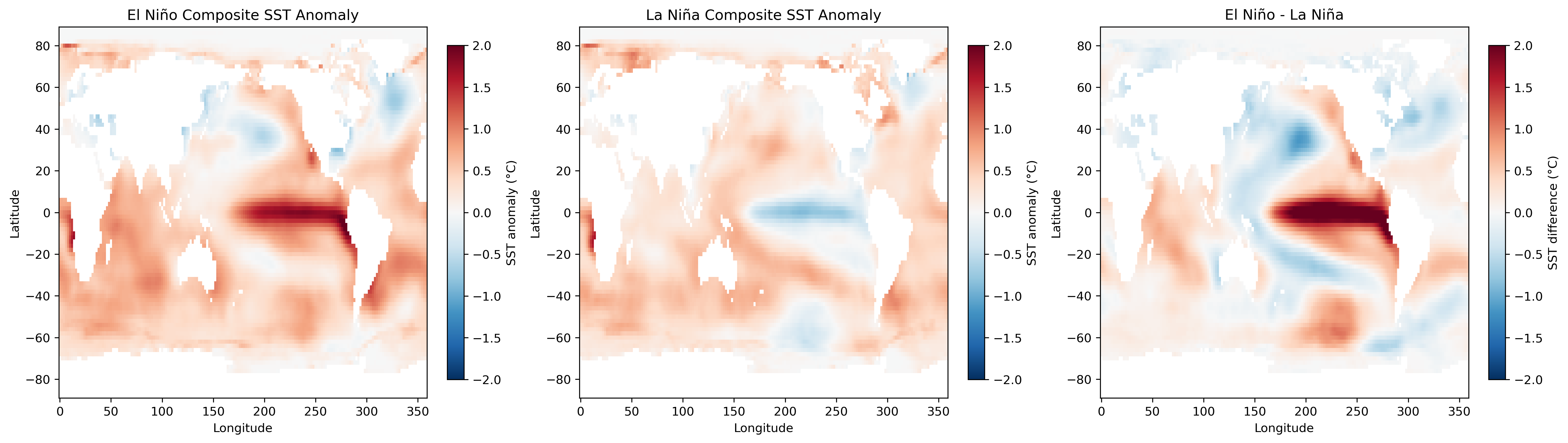
print(f"Saved: {fig_comp_name}")15. SST anomaly コンポジット図
全期間平均からの偏差として、ENSO に伴う空間パターンをより見やすく描く。
# =========================================================
# 10. anomaly コンポジット図
# =========================================================
fig, axes = plt.subplots(1, 3, figsize=(18, 5), constrained_layout=True)

pcm1 = axes[0].pcolormesh(
    comp_el_anom["lon"], comp_el_anom["lat"], comp_el_anom,
    shading="auto", cmap="RdBu_r", vmin=-2, vmax=2
)
axes[0].set_title("El Niño Composite SST Anomaly")
axes[0].set_xlabel("Longitude")
axes[0].set_ylabel("Latitude")
fig.colorbar(pcm1, ax=axes[0], shrink=0.9, label="SST anomaly (°C)")

pcm2 = axes[1].pcolormesh(
    comp_la_anom["lon"], comp_la_anom["lat"], comp_la_anom,
    shading="auto", cmap="RdBu_r", vmin=-2, vmax=2
)
axes[1].set_title("La Niña Composite SST Anomaly")
axes[1].set_xlabel("Longitude")
axes[1].set_ylabel("Latitude")
fig.colorbar(pcm2, ax=axes[1], shrink=0.9, label="SST anomaly (°C)")

pcm3 = axes[2].pcolormesh(
    comp_diff["lon"], comp_diff["lat"], comp_diff,
    shading="auto", cmap="RdBu_r", vmin=-2, vmax=2
)
axes[2].set_title("El Niño - La Niña")
axes[2].set_xlabel("Longitude")
axes[2].set_ylabel("Latitude")
fig.colorbar(pcm3, ax=axes[2], shrink=0.9, label="SST difference (°C)")

plt.savefig(fig_anom_name, dpi=300, bbox_inches="tight", facecolor="white")
plt.show()

print(f"Saved: {fig_anom_name}")
16. 実行結果の例
17. 考察
absolute SST は緯度による平均的な温度差が強く出る。一方、anomaly にすると、全期間平均からのずれを見るため、ENSO に伴う赤道太平洋の暖水・冷水パターンが見えやすくなる。
- なぜ absolute SST より anomaly の方が ENSO 信号を見やすいのか。
- 赤道太平洋以外にも変化が出るのはなぜか。
- このコンポジットから長期トレンドまで説明できるか。
18. まとめ
- Niño3.4 anomaly から ENSO イベント月を判定した。
- 年月単位で Niño 指数と SST を対応付けた。
- イベント月だけの SST を平均し、El Niño / La Niña の代表的パターンを可視化した。
- absolute SST と anomaly では見えるものが違う。
19. 解答の表示
パスワードを入力すると、穴埋めなしの完全スクリプトを表示する。この完全スクリプトは、Jupyter Lab の結果である 08ENSOcomposite.html のコードと一致する。