1. 背景:SLAから何がわかるか
前回までは、海面高度偏差(SLA)を使ってENSOや長期トレンドを調べた。 今回はSLAの空間勾配から地衡流を計算し、海の流れの構造を可視化する。
海面高度が高い場所と低い場所があると、圧力傾度力が生じる。地球が回転しているため、 大規模な海洋ではこの圧力傾度力とコリオリ力がほぼ釣り合い、地衡流が生じる。
今回の狙いは、黒潮、黒潮続流、東北沖の暖水塊を「高さの偏差」だけでなく、「流れ」「回転」「渦活動」として見ることである。
2. 地衡流・相対渦度・EKEの式
SLAを η、重力加速度を g、コリオリパラメータを f とすると、SLA由来の地衡流は次のように書ける。
ug = −(g/f) ∂η/∂y
vg = (g/f) ∂η/∂x
vg = (g/f) ∂η/∂x
ここで、ug は東向き流速、vg は北向き流速である。
ζ = ∂vg/∂x − ∂ug/∂y
ζ は相対渦度で、流れの回転の強さを表す。
EKE = 1/2 (ug2 + vg2)
ここではSLAから計算するため、厳密には「SLA由来の偏差地衡流」と「その運動エネルギー」である。平均流まで含めたい場合は、SLAではなくADTを用いる。
3. 使用データと作成する図
このページと同じディレクトリに次のファイルを置く。
| ファイル | 内容 |
|---|---|
| sla_monthly_0125deg_2024.nc | 2024年1月〜12月の月平均SLA。空間解像度は0.125度。 |
この課題では以下の4枚を作成する。
- 2024年5月のSLAとSLA由来地衡流
- 2024年5月の相対渦度
- 2024年5月のEKE
- 2024年平均EKE
STEP 1
4. ライブラリと設定
import numpy as np
import xarray as xr
import matplotlib.pyplot as plt
import cartopy.crs as ccrs
import cartopy.feature as cfeature

infile = "______________________________.nc"
outfile = "sla_geostrophy_vorticity_eke_japan_2024.nc"

lon_min, lon_max = ______, ______
lat_min, lat_max = ______, ______

month_to_plot = ______
g = ______
omega = ______
Re = ______
ポイント
- cartopy を使うと海岸線や陸地を重ねられる
- 日本周辺を描くため、経度120〜165度、緯度20〜50度を使う
- month_to_plot = 5 とすれば5月の図を描く
STEP 2
5. SLAデータの読み込み
ds = xr.open_dataset(infile)
sla = ds["____"].astype("float64")

sla = sla.sel(
    longitude=slice(lon_min-2, lon_max+2),
    latitude=slice(lat_min-2, lat_max+2)
)

lon = sla["_________"]
lat = sla["________"]

print(sla)
ポイント
- SLAは time, latitude, longitude の3次元配列である
- 勾配計算のため、描画範囲より少し広めに切り出す
- 計算では float64 を使い、保存時に float32 にする
STEP 3
6. 緯度経度を距離に換算する
lat_rad = np.deg2rad(lat)

f = 2 * omega * np.sin(________)
f = xr.DataArray(f, coords={"latitude": lat}, dims=("latitude",))

meters_per_deg_lat = np.pi * Re / 180.0
meters_per_deg_lon = meters_per_deg_lat * np.cos(________)
meters_per_deg_lon = xr.DataArray(
    meters_per_deg_lon,
    coords={"latitude": lat},
    dims=("latitude",)
)
ポイント
- 経度1度あたりの距離は緯度によって変わる
- 高緯度ほど経度方向の距離は短くなる
- 地衡流計算では、度ではなくメートルあたりの勾配が必要である
STEP 4
7. SLA勾配から地衡流を計算する
deta_dlat = sla.differentiate("________") / meters_per_deg_lat
deta_dlon = sla.differentiate("_________") / meters_per_deg_lon

ug = -(g / f) * __________
vg =  (g / f) * __________

ug.name = "ug"
vg.name = "vg"
ug.attrs["units"] = "m s-1"
vg.attrs["units"] = "m s-1"
ポイント
- 南北方向のSLA勾配から東西流速 ug を計算する
- 東西方向のSLA勾配から南北流速 vg を計算する
- 符号を間違えると流れの向きが逆になる
STEP 5
8. 相対渦度とEKEを計算する
dvdx = vg.differentiate("longitude") / meters_per_deg_lon
dudy = ug.differentiate("latitude") / meters_per_deg_lat

zeta = ______ - ______
zeta.name = "relative_vorticity"
zeta.attrs["units"] = "s-1"

zeta_over_f = zeta / ____
zeta_over_f.name = "relative_vorticity_over_f"

eke = 0.5 * ((ug * ______)**2 + (vg * ______)**2)
eke.name = "eke"
eke.attrs["units"] = "cm2 s-2"

log10_mean_eke = np.log10(eke.mean("____"))
ポイント
- 相対渦度は dv/dx - du/dy である
- EKEを cm²/s² で表すため、流速に100を掛けている
- 月ごとのEKEと、2024年平均EKEの両方を描く
STEP 6
9. NetCDFとして保存する
sla_p = sla.sel(longitude=slice(lon_min, lon_max), latitude=slice(lat_min, lat_max))
ug_p = ug.sel(longitude=slice(lon_min, lon_max), latitude=slice(lat_min, lat_max))
vg_p = vg.sel(longitude=slice(lon_min, lon_max), latitude=slice(lat_min, lat_max))
zeta_p = zeta.sel(longitude=slice(lon_min, lon_max), latitude=slice(lat_min, lat_max))
eke_p = eke.sel(longitude=slice(lon_min, lon_max), latitude=slice(lat_min, lat_max))
log10_mean_eke_p = log10_mean_eke.sel(longitude=slice(lon_min, lon_max), latitude=slice(lat_min, lat_max))

out = xr.Dataset({
    "sla": sla_p.astype("float32"),
    "ug": ug_p.astype("float32"),
    "vg": vg_p.astype("float32"),
    "relative_vorticity": zeta_p.astype("float32"),
    "relative_vorticity_over_f": zeta_over_f.sel(
        longitude=slice(lon_min, lon_max),
        latitude=slice(lat_min, lat_max)
    ).astype("float32"),
    "eke": eke_p.astype("float32"),
    "log10_mean_eke": log10_mean_eke_p.astype("float32"),
})

out.to_netcdf(________)
print(f"Saved: {outfile}")
STEP 7
10. 日本周辺で描画する
def plot_map(field, u, v, title, cbar_label,
             vmin=None, vmax=None,
             cmap="turbo", outpng="figure.png",
             vector_step=8,
             contour_sla=None):

    proj = ccrs.PlateCarree()
    fig = plt.figure(figsize=(10, 8))
    ax = plt.axes(projection=proj)
    ax.set_extent([lon_min, lon_max, lat_min, lat_max], crs=proj)

    im = ax.pcolormesh(
        field["longitude"],
        field["latitude"],
        field,
        transform=proj,
        cmap=cmap,
        vmin=vmin,
        vmax=vmax,
        shading="auto"
    )

    ax.coastlines(resolution="10m", linewidth=0.8, zorder=20)
    ax.add_feature(cfeature.LAND, facecolor="lightgray", edgecolor="black", linewidth=0.5, zorder=10)

    if contour_sla is not None:
        cs = ax.contour(
            contour_sla["longitude"],
            contour_sla["latitude"],
            contour_sla,
            levels=np.arange(-1.0, 1.05, 0.1),
            colors="k",
            linewidths=0.45,
            alpha=0.55,
            transform=proj
        )

    uu = u.isel(latitude=slice(None, None, vector_step),
                longitude=slice(None, None, vector_step))
    vv = v.isel(latitude=slice(None, None, vector_step),
                longitude=slice(None, None, vector_step))

    speed = np.sqrt(uu**2 + vv**2)
    mask = speed > ______

    q = ax.quiver(
        uu["longitude"], uu["latitude"],
        uu.where(mask), vv.where(mask),
        transform=proj,
        color="k",
        scale=13,
        width=0.0014,
        alpha=0.70,
        zorder=30
    )

    ax.quiverkey(
        q,
        X=0.08, Y=0.87,
        U=______,
        label="0.5 m/s",
        labelpos="E",
        coordinates="axes",
        fontproperties={"size": 12, "weight": "bold"}
    )

    gl = ax.gridlines(draw_labels=True, linewidth=0.5, alpha=0.45)
    gl.top_labels = False
    gl.right_labels = False

    ax.set_title(title, fontsize=18, weight="bold")
    cb = plt.colorbar(im, ax=ax, orientation="vertical", pad=0.02)
    cb.set_label(cbar_label)

    plt.tight_layout()
    plt.savefig(outpng, dpi=300, bbox_inches="tight", facecolor="white")
    plt.show()
ポイント
- quiverkey によって、ベクトルの基準流速を表示する
- ここではマスクを0にして、すべての流速ベクトルを表示する
- 黒潮続流と東北沖暖水塊を見やすくするため、SLA等値線も重ねる
作成例
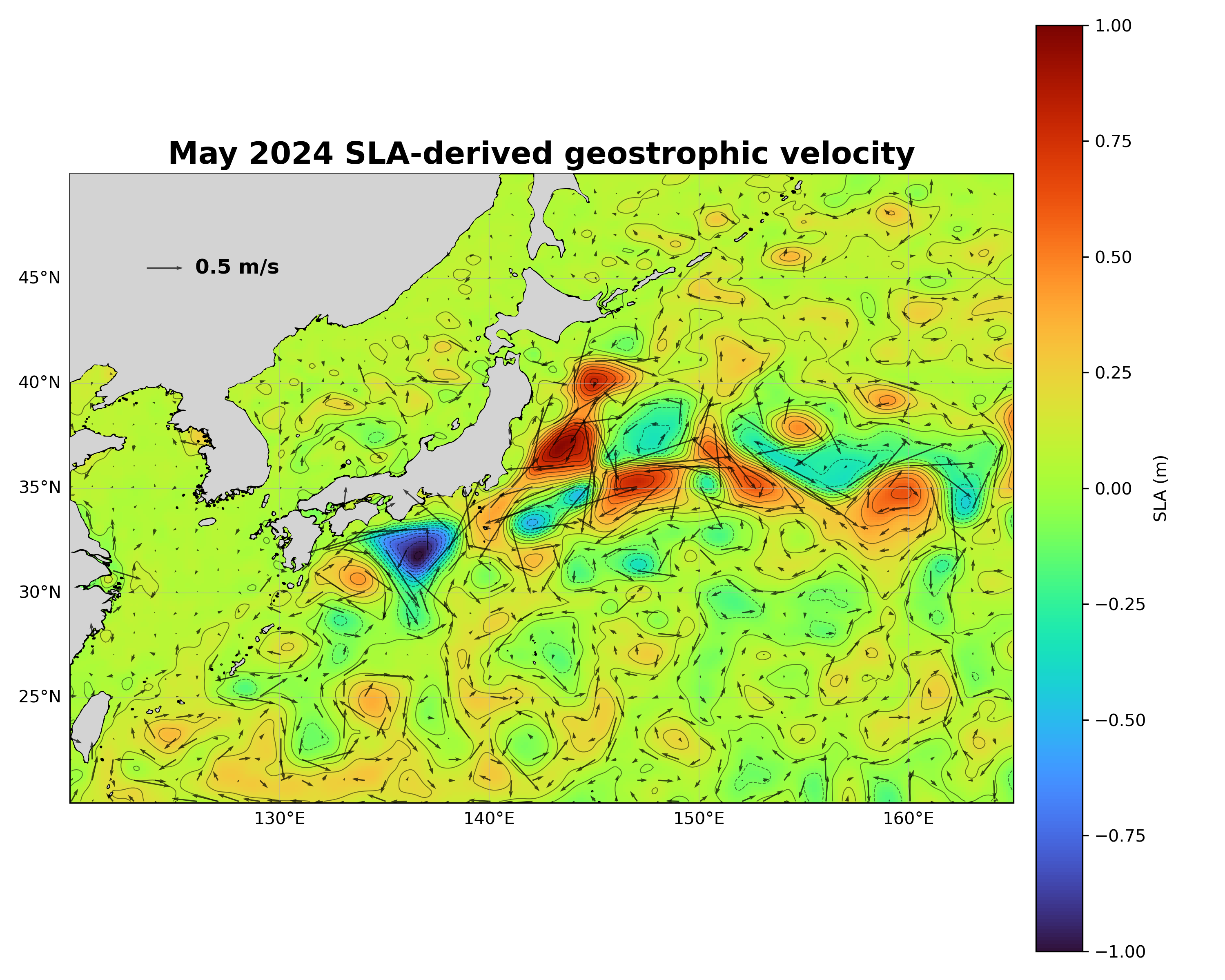
2024年5月のSLAとSLA由来地衡流。黒潮続流と暖水塊にともなう流れが見える。
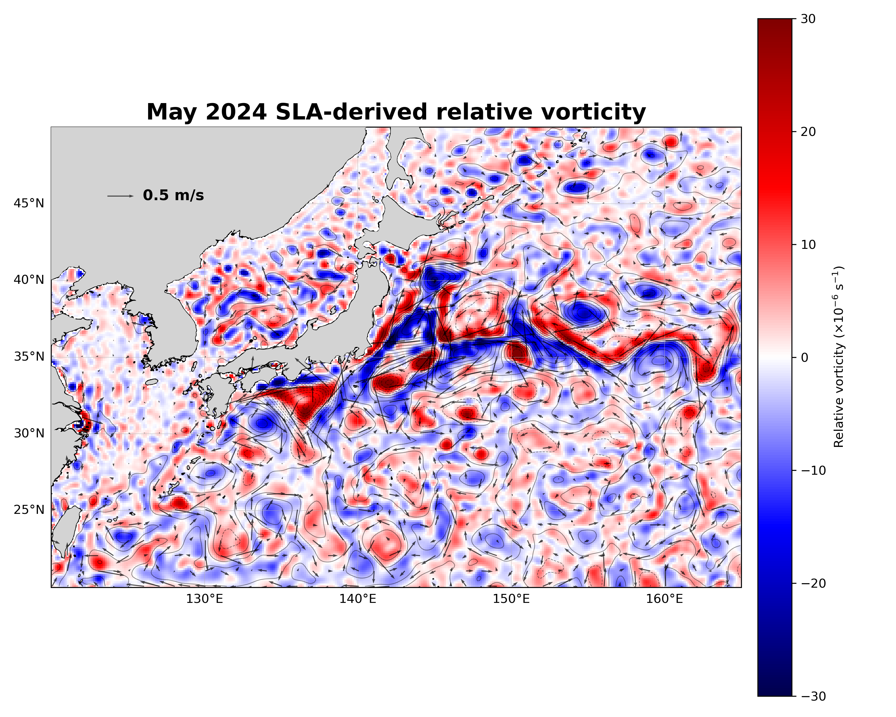
2024年5月の相対渦度。暖水塊・冷水塊の周辺で正負の渦度が強く現れる。
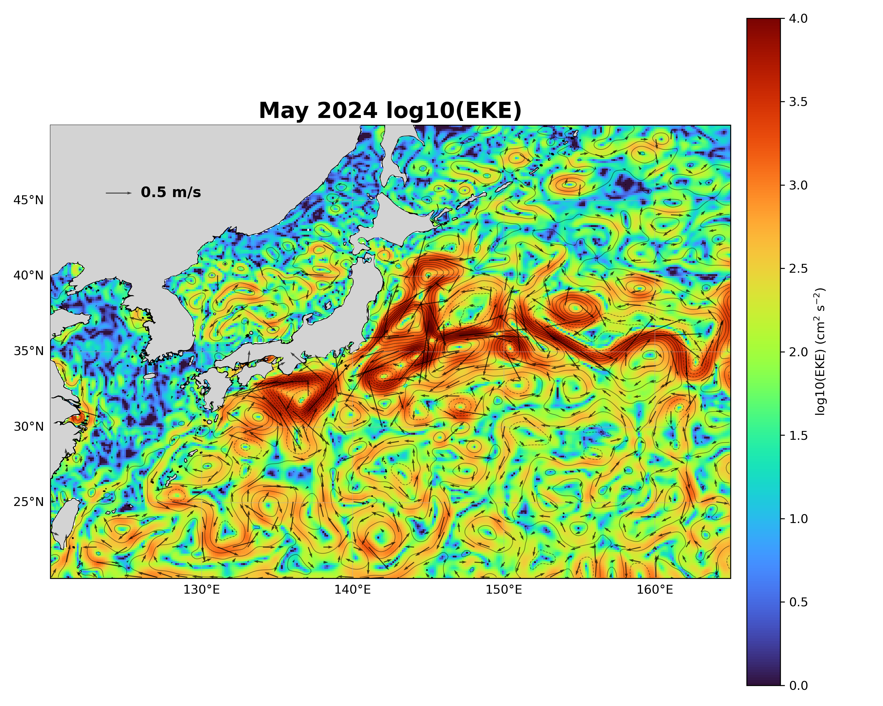
2024年5月のEKE。黒潮・黒潮続流域で渦運動エネルギーが大きい。
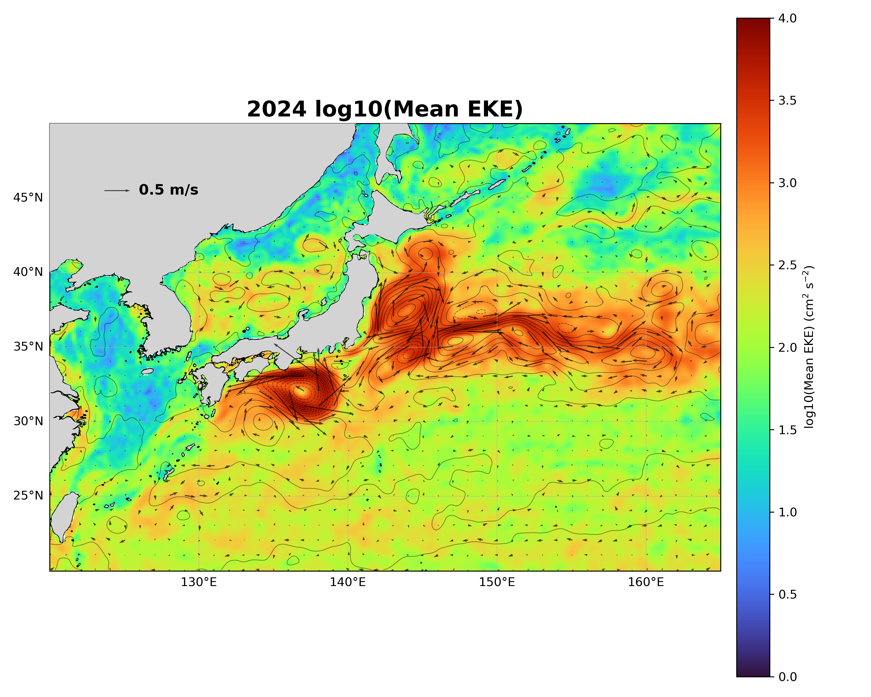
2024年平均EKE。月ごとのノイズがならされ、黒潮続流域の高EKE帯が明瞭になる。
11. 考察課題
考察せよ
- 黒潮・黒潮続流は、SLAの高低差とどのように対応しているか。
- 東北沖の暖水塊では、SLA、流速ベクトル、相対渦度はどのような関係になっているか。
- 相対渦度図で、正の渦度と負の渦度はどのような場所に現れているか。
- 月平均EKEと年平均EKEでは、どちらが黒潮続流域の渦活動帯を説明しやすいか。
- SLA由来の地衡流と、ADT由来の地衡流では何が違うと考えられるか。
SLA由来の地衡流は、平均流そのものではなく偏差流を表す。黒潮の平均的な流路をより直接的に見たい場合は、ADTを用いた同じ計算を行う必要がある。
12. 解答の表示
課題提出後、確認用としてパスワードを入力すると、穴埋めの要点と完全スクリプトを表示する。
穴埋めの要点
sla_monthly_0125deg_2024
120, 165
20, 50
5
9.80665
7.2921e-5
6371000.0
sla
longitude
latitude
lat_rad
lat_rad
latitude
longitude
deta_dlat
deta_dlon
dvdx, dudy
f
100.0, 100.0
time
outfile
0
0.5
完全スクリプト
import numpy as np
import xarray as xr
import matplotlib.pyplot as plt
import cartopy.crs as ccrs
import cartopy.feature as cfeature

# =========================
# Settings
# =========================
infile = "sla_monthly_0125deg_2024.nc"
outfile = "sla_geostrophy_vorticity_eke_japan_2024.nc"

lon_min, lon_max = 120, 165
lat_min, lat_max = 20, 50

month_to_plot = 5

g = 9.80665
omega = 7.2921e-5
Re = 6371000.0

# =========================
# Read SLA
# =========================
ds = xr.open_dataset(infile)
sla = ds["sla"].astype("float64")

sla = sla.sel(
    longitude=slice(lon_min-2, lon_max+2),
    latitude=slice(lat_min-2, lat_max+2)
)

lon = sla["longitude"]
lat = sla["latitude"]

# =========================
# Metric and Coriolis
# =========================
lat_rad = np.deg2rad(lat)

f = 2 * omega * np.sin(lat_rad)
f = xr.DataArray(f, coords={"latitude": lat}, dims=("latitude",))

meters_per_deg_lat = np.pi * Re / 180.0
meters_per_deg_lon = meters_per_deg_lat * np.cos(lat_rad)
meters_per_deg_lon = xr.DataArray(
    meters_per_deg_lon,
    coords={"latitude": lat},
    dims=("latitude",)
)

# =========================
# SLA gradients
# =========================
deta_dlat = sla.differentiate("latitude") / meters_per_deg_lat
deta_dlon = sla.differentiate("longitude") / meters_per_deg_lon

# =========================
# SLA-derived geostrophic velocity
# =========================
ug = -(g / f) * deta_dlat
vg =  (g / f) * deta_dlon

ug.name = "ug"
vg.name = "vg"
ug.attrs["units"] = "m s-1"
vg.attrs["units"] = "m s-1"

# =========================
# Relative vorticity
# =========================
dvdx = vg.differentiate("longitude") / meters_per_deg_lon
dudy = ug.differentiate("latitude") / meters_per_deg_lat

zeta = dvdx - dudy
zeta.name = "relative_vorticity"
zeta.attrs["units"] = "s-1"

zeta_over_f = zeta / f
zeta_over_f.name = "relative_vorticity_over_f"
zeta_over_f.attrs["units"] = "1"

# =========================
# EKE
# =========================
eke = 0.5 * ((ug * 100.0)**2 + (vg * 100.0)**2)
eke.name = "eke"
eke.attrs["units"] = "cm2 s-2"

log10_mean_eke = np.log10(eke.mean("time"))
log10_mean_eke.name = "log10_mean_eke"

# =========================
# Trim region and save
# =========================
sla_p = sla.sel(longitude=slice(lon_min, lon_max), latitude=slice(lat_min, lat_max))
ug_p = ug.sel(longitude=slice(lon_min, lon_max), latitude=slice(lat_min, lat_max))
vg_p = vg.sel(longitude=slice(lon_min, lon_max), latitude=slice(lat_min, lat_max))
zeta_p = zeta.sel(longitude=slice(lon_min, lon_max), latitude=slice(lat_min, lat_max))
eke_p = eke.sel(longitude=slice(lon_min, lon_max), latitude=slice(lat_min, lat_max))
log10_mean_eke_p = log10_mean_eke.sel(longitude=slice(lon_min, lon_max), latitude=slice(lat_min, lat_max))

out = xr.Dataset({
    "sla": sla_p.astype("float32"),
    "ug": ug_p.astype("float32"),
    "vg": vg_p.astype("float32"),
    "relative_vorticity": zeta_p.astype("float32"),
    "relative_vorticity_over_f": zeta_over_f.sel(
        longitude=slice(lon_min, lon_max),
        latitude=slice(lat_min, lat_max)
    ).astype("float32"),
    "eke": eke_p.astype("float32"),
    "log10_mean_eke": log10_mean_eke_p.astype("float32"),
})
out.to_netcdf(outfile)
print(f"Saved: {outfile}")

# =========================
# Plot helper
# =========================
def plot_map(field, u, v, title, cbar_label,
             vmin=None, vmax=None,
             cmap="turbo", outpng="figure.png",
             vector_step=8,
             contour_sla=None):

    proj = ccrs.PlateCarree()
    fig = plt.figure(figsize=(10, 8))
    ax = plt.axes(projection=proj)
    ax.set_extent([lon_min, lon_max, lat_min, lat_max], crs=proj)

    im = ax.pcolormesh(
        field["longitude"],
        field["latitude"],
        field,
        transform=proj,
        cmap=cmap,
        vmin=vmin,
        vmax=vmax,
        shading="auto"
    )

    ax.coastlines(resolution="10m", linewidth=0.8, zorder=20)
    ax.add_feature(cfeature.LAND, facecolor="lightgray", edgecolor="black", linewidth=0.5, zorder=10)

    if contour_sla is not None:
        ax.contour(
            contour_sla["longitude"],
            contour_sla["latitude"],
            contour_sla,
            levels=np.arange(-1.0, 1.05, 0.1),
            colors="k",
            linewidths=0.45,
            alpha=0.55,
            transform=proj
        )

    uu = u.isel(latitude=slice(None, None, vector_step),
                longitude=slice(None, None, vector_step))
    vv = v.isel(latitude=slice(None, None, vector_step),
                longitude=slice(None, None, vector_step))

    speed = np.sqrt(uu**2 + vv**2)
    mask = speed > 0

    q = ax.quiver(
        uu["longitude"], uu["latitude"],
        uu.where(mask), vv.where(mask),
        transform=proj,
        color="k",
        scale=13,
        width=0.0014,
        alpha=0.70,
        zorder=30
    )

    ax.quiverkey(
        q,
        X=0.08, Y=0.87,
        U=0.5,
        label="0.5 m/s",
        labelpos="E",
        coordinates="axes",
        fontproperties={"size": 12, "weight": "bold"}
    )

    gl = ax.gridlines(draw_labels=True, linewidth=0.5, alpha=0.45)
    gl.top_labels = False
    gl.right_labels = False

    ax.set_title(title, fontsize=18, weight="bold")
    cb = plt.colorbar(im, ax=ax, orientation="vertical", pad=0.02)
    cb.set_label(cbar_label)

    plt.tight_layout()
    plt.savefig(outpng, dpi=300, bbox_inches="tight", facecolor="white")
    plt.show()

# =========================
# Figures
# =========================
sla_m = sla_p.isel(time=month_to_plot-1)
ug_m = ug_p.isel(time=month_to_plot-1)
vg_m = vg_p.isel(time=month_to_plot-1)
zeta_m = zeta_p.isel(time=month_to_plot-1)
eke_m = eke_p.isel(time=month_to_plot-1)

plot_map(
    field=sla_m,
    u=ug_m,
    v=vg_m,
    title="May 2024 SLA-derived geostrophic velocity",
    cbar_label="SLA (m)",
    vmin=-1.0,
    vmax=1.0,
    cmap="turbo",
    outpng="fig_japan_sla_gv_may2024.png",
    vector_step=8,
    contour_sla=sla_m
)

plot_map(
    field=zeta_m * 1e6,
    u=ug_m,
    v=vg_m,
    title="May 2024 SLA-derived relative vorticity",
    cbar_label="Relative vorticity (×10$^{-6}$ s$^{-1}$)",
    vmin=-30,
    vmax=30,
    cmap="seismic",
    outpng="fig_japan_relative_vorticity_may2024.png",
    vector_step=8,
    contour_sla=sla_m
)

plot_map(
    field=np.log10(eke_m),
    u=ug_m,
    v=vg_m,
    title="May 2024 log10(EKE)",
    cbar_label="log10(EKE) (cm$^2$ s$^{-2}$)",
    vmin=0,
    vmax=4,
    cmap="turbo",
    outpng="fig_japan_log10_eke_may2024.png",
    vector_step=8,
    contour_sla=sla_m
)

mean_ug = ug_p.mean("time")
mean_vg = vg_p.mean("time")

plot_map(
    field=log10_mean_eke_p,
    u=mean_ug,
    v=mean_vg,
    title="2024 log10(Mean EKE)",
    cbar_label="log10(Mean EKE) (cm$^2$ s$^{-2}$)",
    vmin=0,
    vmax=4,
    cmap="turbo",
    outpng="fig_japan_log10_mean_eke_2024.png",
    vector_step=8,
    contour_sla=sla_p.mean("time")
)