1. 背景:クロロフィルの季節変動を見る
前回は、SGLIの1時期のクロロフィル分布を地図にした。今回は、1枚の地図ではなく、12か月の気候値を使って「季節変動のパターン」が似ている海域を分類する。
たとえば、北半球中緯度では春にクロロフィルが高くなることが多い。一方、亜熱帯循環域では年間を通じて低濃度で、赤道域や沿岸域ではまた異なる季節変動を示す。このような違いを、K-means クラスタリングで客観的に分ける。
今回のポイント:1つの格子点を1つのサンプルと考え、12か月のクロロフィル値を12個の特徴量として使う。
2. 使用データ
使用するファイルは、GlobColour の 100 km 解像度の月別 log10 クロロフィル気候値である。太平洋域だけを切り出し、K-means にかける。
| 項目 | 内容 |
|---|---|
| 入力ファイル | GlobColour_log10CHL1_clim12_100km_AV_199709_202603.nc |
| 変数名 | log10_chl_clim(month, lat, lon) |
| 対象範囲 | 太平洋域:120E–280E, 60S–60N |
| 主な処理 | raw log10(CHL) による分類、季節変動形状による分類、K=3〜6の比較 |
注意:このデータでは経度を 0–360 表記で扱う。つまり 280E は 80W に相当する。
3. K-meansで何を分類するのか
K-means は、似た特徴を持つデータを K 個のグループに分ける方法である。ここでは、各格子点の12か月のクロロフィル値をベクトルとして扱う。
1つの格子点 = [1月, 2月, 3月, ..., 12月] の12個の値今回は2通りの分類を行う。
- raw log10(CHL):クロロフィル濃度の高低と季節変動の両方で分類する。
- seasonal-cycle shape:各格子点で平均を引き、標準偏差で割ることで、濃度の高低ではなく季節変動の形で分類する。
X_shape = (X - 12か月平均) / 12か月標準偏差この標準化により、「濃い海域・薄い海域」ではなく、「何月に高く、何月に低いか」が似ている海域を探せる。
4. 作成される図の例
4.1 元データの確認
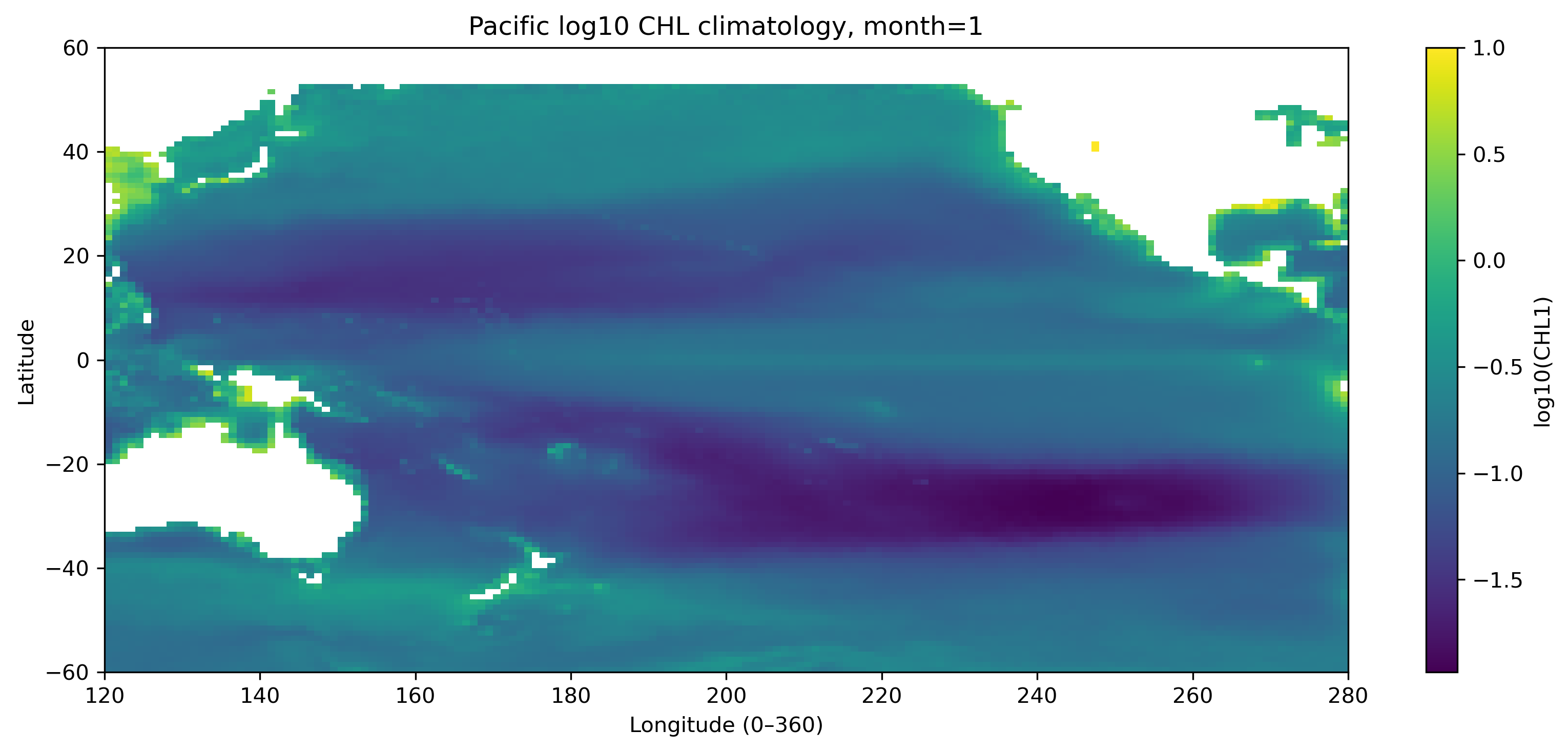
図1. 太平洋域の log10 クロロフィル気候値(1月)。
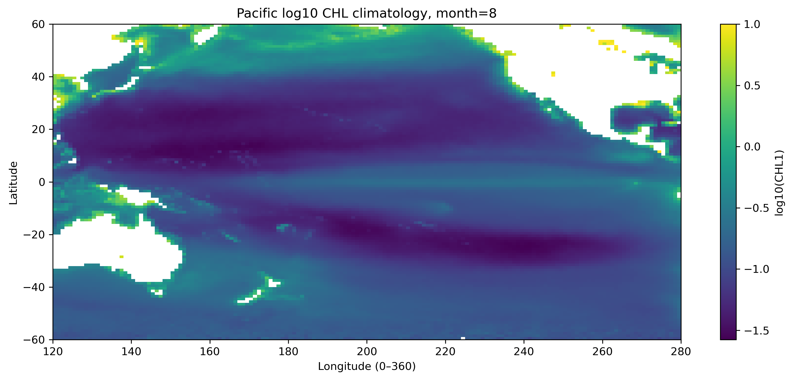
図2. 太平洋域の log10 クロロフィル気候値(8月)。北半球・南半球で季節変化が異なることに注目する。
4.2 raw log10(CHL) による分類
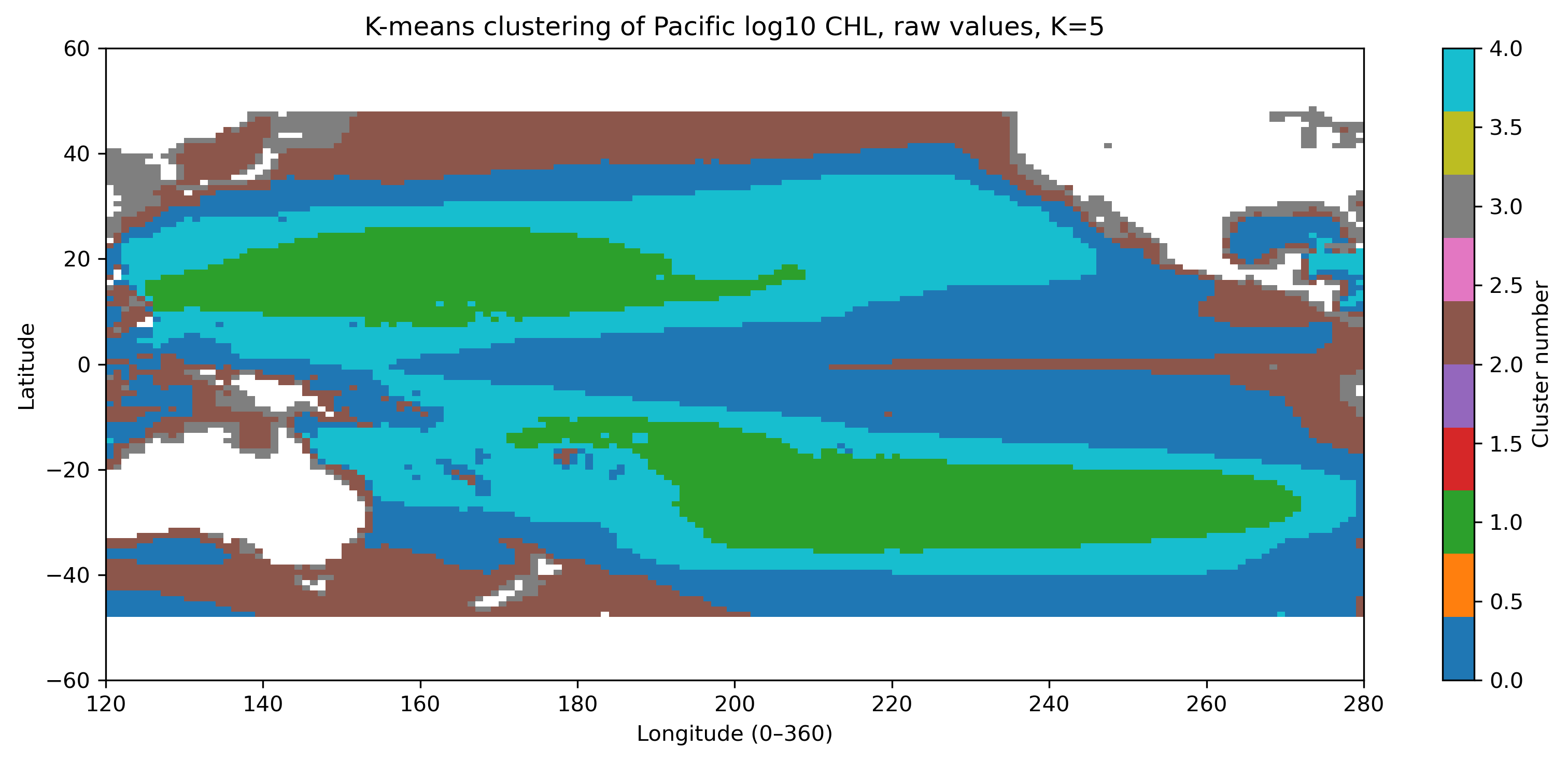
図3. raw log10(CHL) をそのまま使った K-means 分類(K=5)。濃度の高低の影響を強く受ける。
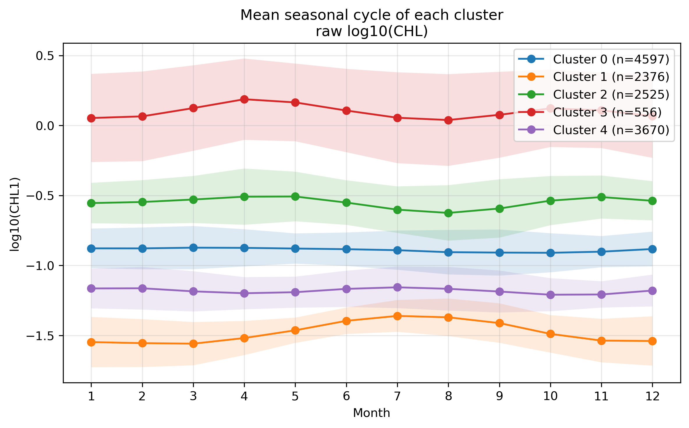
図4. raw log10(CHL) 分類における各クラスタの平均季節変化。
4.3 季節変動の形による分類

図5. 各格子点で標準化した季節変動の形に基づく分類(K=5)。
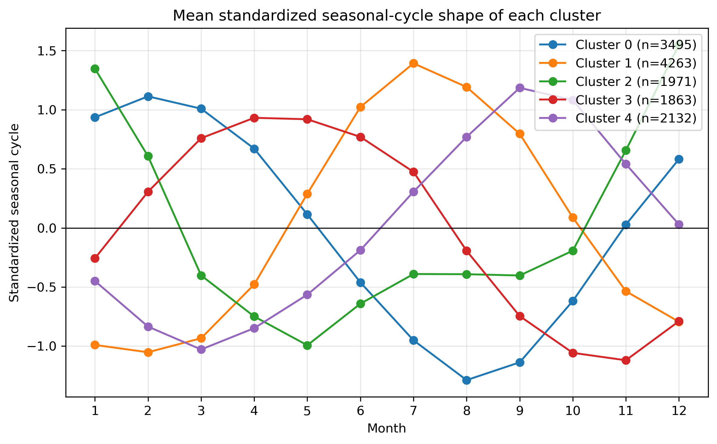
図6. 標準化後の平均季節変動。濃度の大小ではなく、何月に相対的に高いかを比較する。
4.4 Kを変えたときの比較
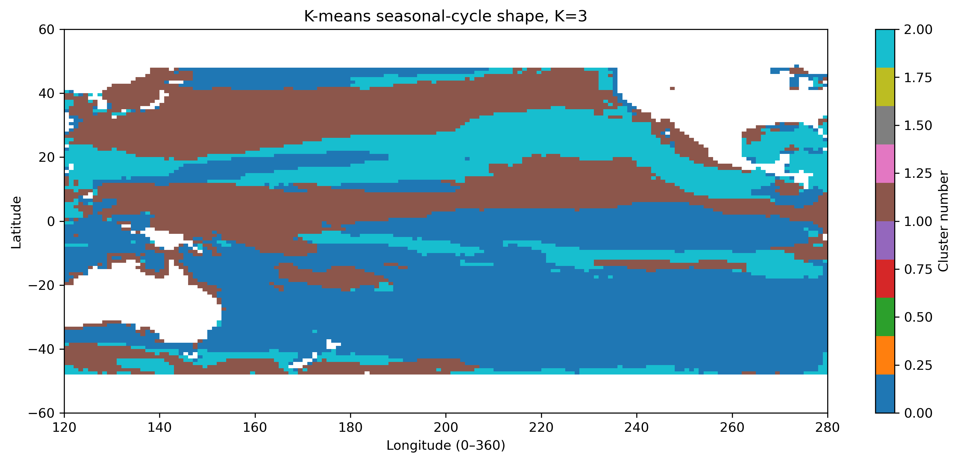
図7. 季節変動形状クラスタリング K=3。
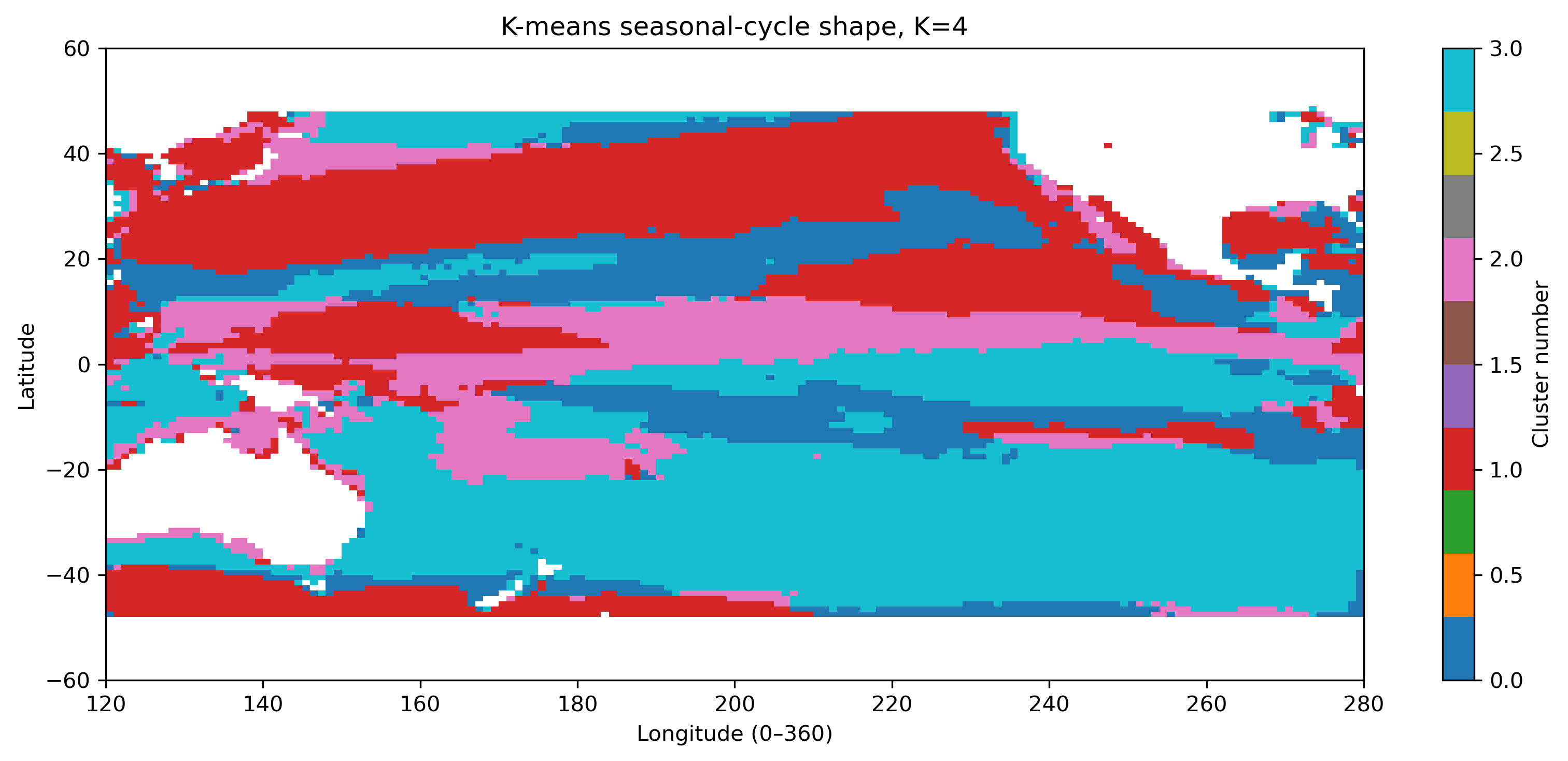
図8. 季節変動形状クラスタリング K=4。
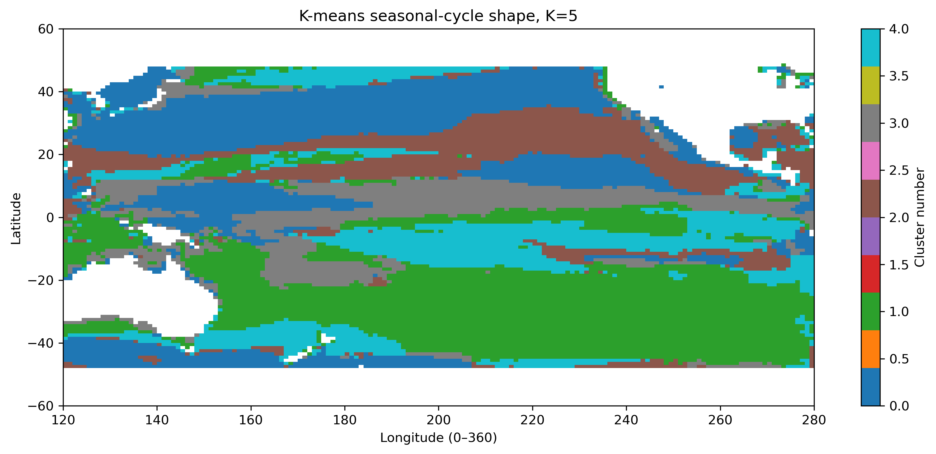
図9. 季節変動形状クラスタリング K=5。
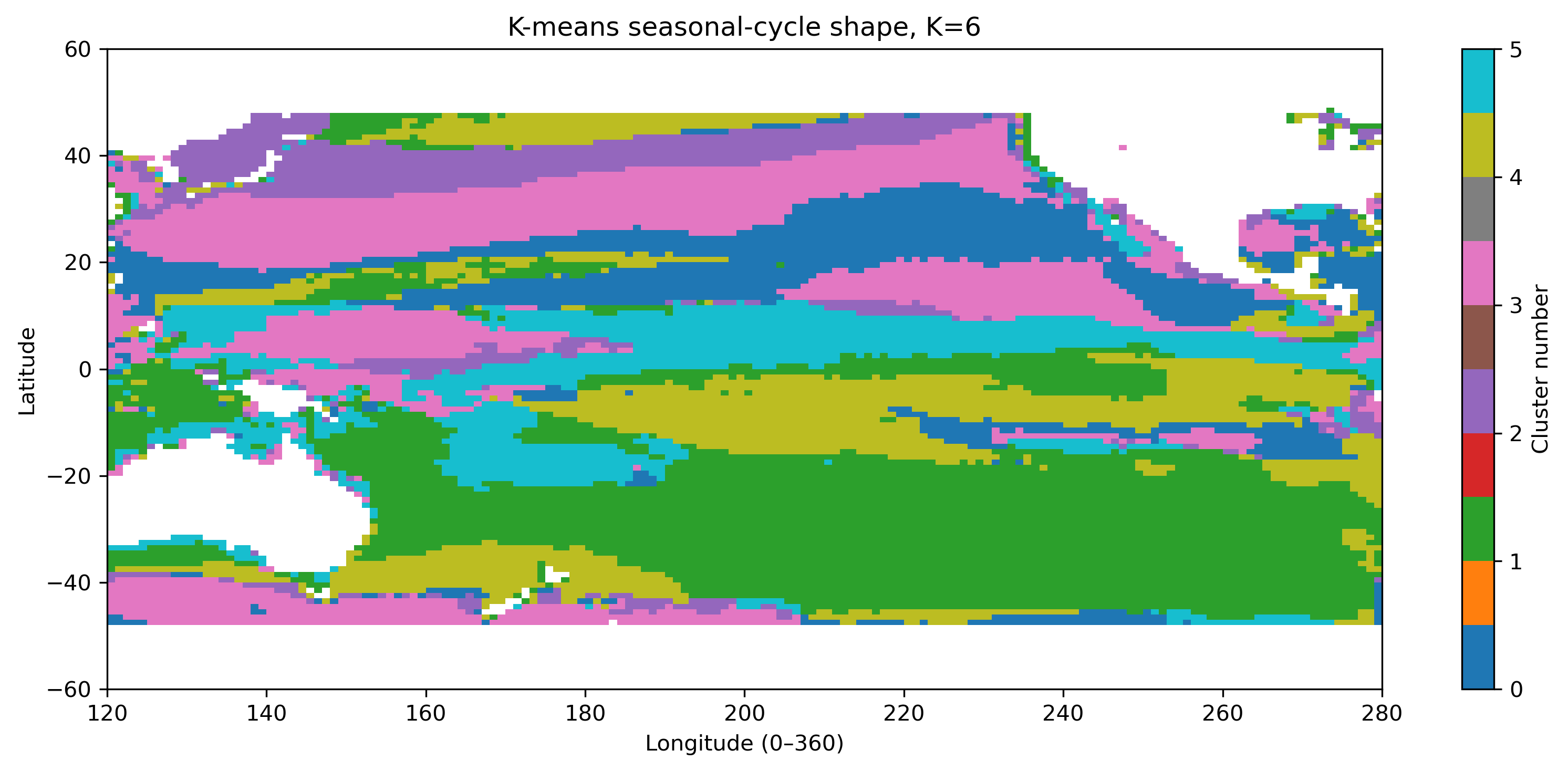
図10. 季節変動形状クラスタリング K=6。
4.5 平均季節変動の比較
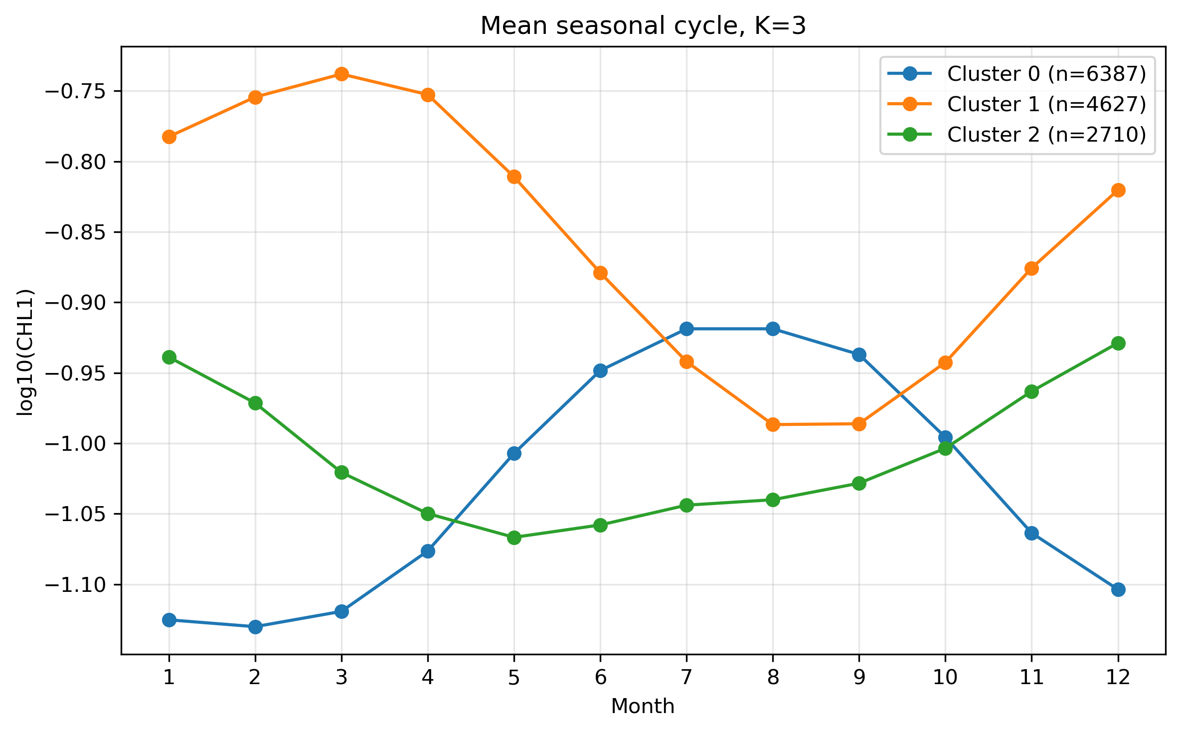
図11. K=3 の平均季節変化。
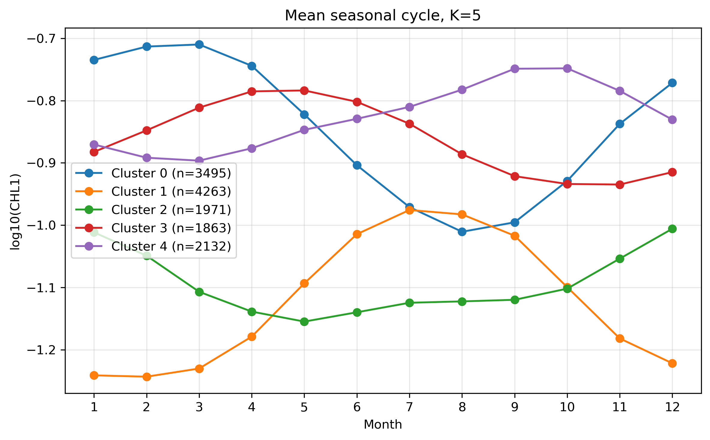
図12. K=5 の平均季節変化。
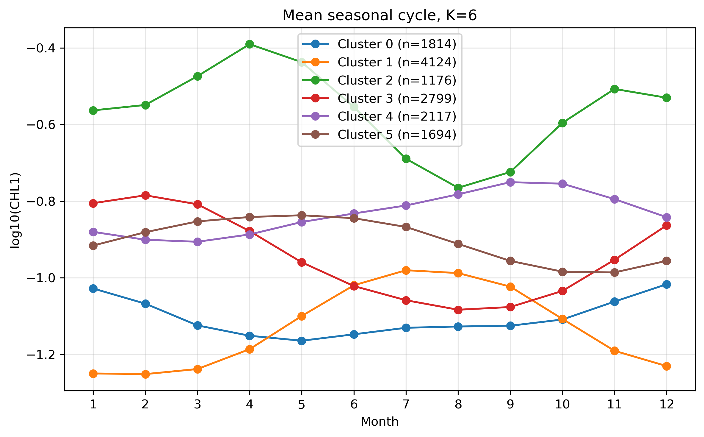
図13. K=6 の平均季節変化。
図の保存:このページのスクリプトでは、Jupyter Labで表示した図を figures_14_clustering_chl100km/ に PNG として保存する。
5. 穴埋めポイント
以下の空欄 ____ を埋めながら、処理の意味を確認する。
STEP 1:設定
from pathlib import Path
import numpy as np
import xarray as xr
import matplotlib.pyplot as plt
from sklearn.cluster import KMeans

base_dir = Path("____")
ncfile = base_dir / "____"
K = ____
lat_min, lat_max = ____, ____
lon_min, lon_max = ____, ____
STEP 2:データを読み、緯度経度を整える
ds = xr.open_dataset(ncfile)
chl = ds["____"]
chl = chl.sortby("____")
lon_360 = (chl["lon"] + ____) % ____
chl = chl.assign_coords(____=lon_360)
chl = chl.sortby("____")
STEP 3:太平洋域を切り出し、K-means用の行列を作る
chl_pac = chl.sel(
    lat=slice(____, ____),
    lon=slice(____, ____)
)

chl_for_cluster = chl_pac.transpose("____", "____", "____")
A = chl_for_cluster.values
X = A.reshape(____ * ____, ____)
valid = np.isfinite(X).all(axis=____)
X_valid = X[valid, :]
STEP 4:raw log10(CHL) でクラスタリングする
kmeans_raw = KMeans(n_clusters=____, random_state=0, n_init=20)
labels_raw = kmeans_raw.fit_predict(X_valid)
STEP 5:季節変動の形でクラスタリングする
X_mean = np.nanmean(X_valid, axis=____, keepdims=True)
X_std  = np.nanstd(X_valid,  axis=____, keepdims=True)
X_shape = (X_valid2 - ____) / ____

kmeans_shape = KMeans(n_clusters=____, random_state=0, n_init=20)
labels_shape = kmeans_shape.fit_predict(X_shape)
6. 穴埋め版・完全スクリプト
以下を Jupyter Lab のセルにそのまま貼り付け、____ を埋めてから実行する。図は表示されるだけでなく、PNGとして保存される。
# ============================================================
# 14. GlobColour 100 km log10 CHL 12か月気候値を用いた
#     太平洋域 K-means クラスタリング 完全スクリプト
# ============================================================
#
# このスクリプトで行うこと
# 1. GlobColour の 100 km log10(CHL) 12か月気候値 NetCDF を読む
# 2. 太平洋域 120E–280E, 60S–60N を切り出す
# 3. K-means 用に (格子点, 12か月) のデータ行列を作る
# 4. raw log10(CHL) によるクラスタリングを行う
# 5. 季節変動の形を標準化してクラスタリングを行う
# 6. K=3,4,5,6 の比較を行う
# 7. NetCDF と PNG 図を保存する
#
# 入力ファイル:
#   GlobColour_log10CHL1_clim12_100km_AV_199709_202603.nc
#
# 出力:
#   GlobColour_Kmeans_cluster_K5_Pacific_100km.nc
#   figures_14_clustering_chl100km/*.png
# ============================================================

import numpy as np
import xarray as xr
import matplotlib.pyplot as plt

from pathlib import Path
from sklearn.cluster import KMeans


# ============================================================
# 0. 設定
# ============================================================
#
# Jupyter Lab でこのノートブックを実行している作業ディレクトリに
# NetCDFファイルを置く場合は、base_dir = Path(".") でもよい。
# 先生の環境で絶対パスを使う場合は、下のように指定する。
# ============================================================

base_dir = Path("____")  # 作業ディレクトリを使う場合は "."

ncfile = base_dir / "____"  # 入力NetCDFファイル名

# 図の保存先
figdir = base_dir / "figures_14_clustering_chl100km"
figdir.mkdir(parents=True, exist_ok=True)

# クラスタ数
K = ____  # まずは 5

# 太平洋域の切り出し範囲
lat_min = ____  # -60
lat_max = ____   # 60

# 経度は 0〜360 表記で扱う
# 120E = 120, 80W = 280
lon_min = ____  # 120
lon_max = ____  # 280

print("Input file:")
print(ncfile)
print("Exists:", ncfile.exists())
print("Figure directory:")
print(figdir)

if not ncfile.exists():
    raise FileNotFoundError(f"ファイルが見つかりません: {ncfile}")


# ============================================================
# 図保存用の小さな関数
# ============================================================

def save_current_figure(filename):
    """
    現在の図をPNGとして保存する。
    Jupyter Lab上では表示もしたいので、この関数の後に plt.show() する。
    """
    out_png = figdir / filename
    plt.savefig(
        out_png,
        dpi=300,
        bbox_inches="tight",
        facecolor="white"
    )
    print("Saved figure:", out_png)


# ============================================================
# 1. データを読む
# ============================================================

ds = xr.open_dataset(ncfile)

print("\n===== Original dataset =====")
print(ds)

chl = ds["____"]  # log10_chl_clim

print("\n===== Original variable =====")
print(chl)
print("dims :", chl.dims)
print("shape:", chl.shape)

print("\nOriginal lat range:",
      float(chl["lat"].min()), float(chl["lat"].max()))
print("Original lon range:",
      float(chl["lon"].min()), float(chl["lon"].max()))


# ============================================================
# 2. 緯度を昇順にそろえる
# ============================================================
#
# データによっては lat が 90 -> -90 の順になっている。
# slice(-60, 60) を安全に使うため、lat を昇順にする。
# ============================================================

chl = chl.sortby("____")  # lat

print("\nAfter sorting latitude:")
print("lat range:",
      float(chl["lat"].min()), float(chl["lat"].max()))


# ============================================================
# 3. 経度を 0〜360 に変換する
# ============================================================
#
# 例:
#   -80  -> 280
#   -170 -> 190
#   120  -> 120
#
# これにより、太平洋を 120E〜280E として連続的に扱える。
# ============================================================

lon_original = chl["lon"]
lon_360 = (lon_original + ____) % ____  # 360, 360

chl = chl.assign_coords(____=lon_360)  # lon

# 経度方向に並べ替える
chl = chl.sortby("____")  # lon

print("\nAfter converting lon to 0-360:")
print("lon range:",
      float(chl["lon"].min()), float(chl["lon"].max()))


# ============================================================
# 4. 太平洋域を切り出す
# ============================================================
#
# 緯度:60S〜60N
# 経度:120E〜280E
# 280E は 80W に相当する。
# ============================================================

chl_pac = chl.sel(
    lat=slice(____, ____)  # lat_min, lat_max,
    lon=slice(____, ____)  # lon_min, lon_max
)

print("\n===== Pacific subset =====")
print(chl_pac)
print("Pacific lat range:",
      float(chl_pac["lat"].min()), float(chl_pac["lat"].max()))
print("Pacific lon range:",
      float(chl_pac["lon"].min()), float(chl_pac["lon"].max()))
print("Pacific shape:", chl_pac.shape)


# ============================================================
# 5. 太平洋だけになっているか図で確認
# ============================================================

for m in [1, 8]:
    da = chl_pac.sel(month=m)

    plt.figure(figsize=(11, 5))
    plt.pcolormesh(
        chl_pac["lon"],
        chl_pac["lat"],
        da,
        shading="auto"
    )
    plt.colorbar(label="log10(CHL1)")
    plt.xlabel("Longitude (0–360)")
    plt.ylabel("Latitude")
    plt.title(f"Pacific log10 CHL climatology, month={m}")
    plt.xlim(lon_min, lon_max)
    plt.ylim(lat_min, lat_max)
    plt.tight_layout()

    save_current_figure(f"fig14_01_pacific_log10chl_month{m:02d}.png")
    plt.show()


# ============================================================
# 6. K-means 用のデータ行列を作る
# ============================================================
#
# 元データ:
#   chl_pac(month, lat, lon)
#
# K-means 用:
#   X(grid, month)
#
# つまり、
#   1つの格子点 = 1つのサンプル
#   12か月の値 = 12個の特徴量
# ============================================================

chl_for_cluster = chl_pac.transpose("____", "____", "____")  # lat, lon, month

lat = chl_for_cluster["lat"].values
lon = chl_for_cluster["lon"].values
months = chl_for_cluster["month"].values

nlat = len(lat)
nlon = len(lon)
nmon = len(months)

print("\n===== Array size =====")
print("nlat:", nlat)
print("nlon:", nlon)
print("nmon:", nmon)

A = chl_for_cluster.values            # shape = (lat, lon, month)
X = A.reshape(____ * ____, ____)  # nlat, nlon, nmon      # shape = (grid, month)

print("X shape:", X.shape)


# ============================================================
# 7. 欠損を含む格子点を除外する
# ============================================================
#
# 12か月すべてにデータがある格子点だけを使う。
# ============================================================

valid = np.isfinite(X).all(axis=____)  # 1
X_valid = X[valid, :]

print("\n===== Valid grid points =====")
print("Total grid points  :", X.shape[0])
print("Valid grid points  :", X_valid.shape[0])
print("Invalid grid points:", np.sum(~valid))

if X_valid.shape[0] == 0:
    raise ValueError("有効な格子点がありません。範囲や欠損条件を確認してください。")


# ============================================================
# 8. クラスタリング その1:log10(CHL) をそのまま使う
# ============================================================
#
# 意味:
#   平均濃度の違い + 季節変動の違い
#   の両方で分類する。
# ============================================================

kmeans_raw = KMeans(
    n_clusters=____,  # K
    random_state=0,
    n_init=20
)

labels_raw = kmeans_raw.fit_predict(X_valid)

print("\nK-means raw finished.")
print("Cluster labels:", np.unique(labels_raw))

# ラベルを地図に戻す
label_map_raw_1d = np.full(nlat * nlon, np.nan)
label_map_raw_1d[valid] = labels_raw
label_map_raw = label_map_raw_1d.reshape(nlat, nlon)

# 図示:raw log10(CHL) クラスタ地図
plt.figure(figsize=(11, 5))
plt.pcolormesh(
    lon,
    lat,
    label_map_raw,
    shading="auto",
    cmap="tab10"
)
plt.colorbar(label="Cluster number")
plt.xlabel("Longitude (0–360)")
plt.ylabel("Latitude")
plt.title(f"K-means clustering of Pacific log10 CHL, raw values, K={K}")
plt.xlim(lon_min, lon_max)
plt.ylim(lat_min, lat_max)
plt.tight_layout()

save_current_figure(f"fig14_02_cluster_map_raw_K{K}.png")
plt.show()

# 図示:raw log10(CHL) クラスタの平均季節変動
plt.figure(figsize=(8, 5))

for k in range(K):
    cluster_data = X_valid[labels_raw == k, :]
    mean_cycle = np.nanmean(cluster_data, axis=0)
    std_cycle = np.nanstd(cluster_data, axis=0)

    plt.plot(
        months,
        mean_cycle,
        marker="o",
        label=f"Cluster {k} (n={cluster_data.shape[0]})"
    )
    plt.fill_between(
        months,
        mean_cycle - std_cycle,
        mean_cycle + std_cycle,
        alpha=0.15
    )

plt.xlabel("Month")
plt.ylabel("log10(CHL1)")
plt.title("Mean seasonal cycle of each cluster\nraw log10(CHL)")
plt.xticks(months)
plt.grid(True, alpha=0.3)
plt.legend()
plt.tight_layout()

save_current_figure(f"fig14_03_mean_cycle_raw_K{K}.png")
plt.show()


# ============================================================
# 9. クラスタリング その2:各格子点ごとに季節変動を標準化する
# ============================================================
#
# ここが重要。
#
# 各格子点について、
#   12か月平均を引く
#   12か月標準偏差で割る
#
# こうすると、平均クロロフィル濃度の高低よりも、
# 「季節変動の形」に注目した分類になる。
# ============================================================

X_mean = np.nanmean(X_valid, axis=____, keepdims=True)  # 1
X_std = np.nanstd(X_valid, axis=____, keepdims=True)  # 1

# 標準偏差がゼロの格子点を除く
valid_std = np.squeeze(X_std > 0)

X_valid2 = X_valid[valid_std, :]
X_mean2 = X_mean[valid_std, :]
X_std2 = X_std[valid_std, :]

X_shape = (X_valid2 - ____) / ____  # X_mean2, X_std2

print("\n===== Seasonal-shape standardization =====")
print("Original valid points:", X_valid.shape[0])
print("After std check      :", X_shape.shape[0])
print("X_shape mean:", np.nanmean(X_shape))
print("X_shape std :", np.nanstd(X_shape))

kmeans_shape = KMeans(
    n_clusters=____,  # K
    random_state=0,
    n_init=20
)

labels_shape = kmeans_shape.fit_predict(X_shape)

print("\nK-means seasonal-shape finished.")
print("Cluster labels:", np.unique(labels_shape))

# 地図へ戻す
# 注意:valid の中からさらに valid_std の点だけを使っている。
valid_indices = np.where(valid)[0]
valid_shape_indices = valid_indices[valid_std]

label_map_shape_1d = np.full(nlat * nlon, np.nan)
label_map_shape_1d[valid_shape_indices] = labels_shape
label_map_shape = label_map_shape_1d.reshape(nlat, nlon)

# 図示:季節変動の形に基づくクラスタ地図
plt.figure(figsize=(11, 5))
plt.pcolormesh(
    lon,
    lat,
    label_map_shape,
    shading="auto",
    cmap="tab10"
)
plt.colorbar(label="Cluster number")
plt.xlabel("Longitude (0–360)")
plt.ylabel("Latitude")
plt.title(f"K-means clustering of Pacific CHL seasonal-cycle shape, K={K}")
plt.xlim(lon_min, lon_max)
plt.ylim(lat_min, lat_max)
plt.tight_layout()

save_current_figure(f"fig14_04_cluster_map_shape_K{K}.png")
plt.show()

# 図示:分類は標準化後で行い、元の log10(CHL) で平均季節変動を見る
plt.figure(figsize=(8, 5))

for k in range(K):
    cluster_data = X_valid2[labels_shape == k, :]
    mean_cycle = np.nanmean(cluster_data, axis=0)
    std_cycle = np.nanstd(cluster_data, axis=0)

    plt.plot(
        months,
        mean_cycle,
        marker="o",
        label=f"Cluster {k} (n={cluster_data.shape[0]})"
    )
    plt.fill_between(
        months,
        mean_cycle - std_cycle,
        mean_cycle + std_cycle,
        alpha=0.15
    )

plt.xlabel("Month")
plt.ylabel("log10(CHL1)")
plt.title("Mean seasonal cycle of each cluster\nclassified by seasonal-cycle shape")
plt.xticks(months)
plt.grid(True, alpha=0.3)
plt.legend()
plt.tight_layout()

save_current_figure(f"fig14_05_mean_cycle_shape_original_units_K{K}.png")
plt.show()

# 図示:標準化後の季節変動の形を見る
plt.figure(figsize=(8, 5))

for k in range(K):
    cluster_data = X_shape[labels_shape == k, :]
    mean_cycle = np.nanmean(cluster_data, axis=0)

    plt.plot(
        months,
        mean_cycle,
        marker="o",
        label=f"Cluster {k} (n={cluster_data.shape[0]})"
    )

plt.axhline(0, color="k", linewidth=0.8)
plt.xlabel("Month")
plt.ylabel("Standardized seasonal cycle")
plt.title("Mean standardized seasonal-cycle shape of each cluster")
plt.xticks(months)
plt.grid(True, alpha=0.3)
plt.legend()
plt.tight_layout()

save_current_figure(f"fig14_06_mean_standardized_shape_K{K}.png")
plt.show()


# ============================================================
# 10. K を変えて比較する
# ============================================================
#
# 学生課題ではここが重要。
# K=3,4,5,6 で結果がどう変わるかを見る。
# ここでは「季節変動の形」に基づくクラスタリングだけを比較する。
# ============================================================

K_list = [____, ____, ____, ____]  # 3, 4, 5, 6

for K_test in K_list:
    kmeans_tmp = KMeans(
        n_clusters=K_test,
        random_state=0,
        n_init=20
    )

    labels_tmp = kmeans_tmp.fit_predict(X_shape)

    label_map_tmp_1d = np.full(nlat * nlon, np.nan)
    label_map_tmp_1d[valid_shape_indices] = labels_tmp
    label_map_tmp = label_map_tmp_1d.reshape(nlat, nlon)

    # 図示:Kを変えたクラスタ地図
    plt.figure(figsize=(11, 5))
    plt.pcolormesh(
        lon,
        lat,
        label_map_tmp,
        shading="auto",
        cmap="tab10"
    )
    plt.colorbar(label="Cluster number")
    plt.xlabel("Longitude (0–360)")
    plt.ylabel("Latitude")
    plt.title(f"K-means seasonal-cycle shape, K={K_test}")
    plt.xlim(lon_min, lon_max)
    plt.ylim(lat_min, lat_max)
    plt.tight_layout()

    save_current_figure(f"fig14_07_cluster_map_shape_K{K_test}.png")
    plt.show()

    # 図示:Kを変えた平均季節変動
    plt.figure(figsize=(8, 5))

    for k in range(K_test):
        cluster_data = X_valid2[labels_tmp == k, :]
        mean_cycle = np.nanmean(cluster_data, axis=0)

        plt.plot(
            months,
            mean_cycle,
            marker="o",
            label=f"Cluster {k} (n={cluster_data.shape[0]})"
        )

    plt.xlabel("Month")
    plt.ylabel("log10(CHL1)")
    plt.title(f"Mean seasonal cycle, K={K_test}")
    plt.xticks(months)
    plt.grid(True, alpha=0.3)
    plt.legend()
    plt.tight_layout()

    save_current_figure(f"fig14_08_mean_cycle_shape_K{K_test}.png")
    plt.show()


# ============================================================
# 11. 結果を NetCDF に保存する
# ============================================================

out_cluster = base_dir / f"GlobColour_Kmeans_cluster_K{K}_Pacific_100km.nc"

ds_cluster = xr.Dataset(
    data_vars={
        "cluster_raw": (("lat", "lon"), label_map_raw.astype("float32")),
        "cluster_shape": (("lat", "lon"), label_map_shape.astype("float32")),
    },
    coords={
        "lat": lat.astype("float32"),
        "lon": lon.astype("float32"),
    },
    attrs={
        "title": "K-means clustering result for Pacific GlobColour log10 CHL climatology",
        "description": (
            "Cluster labels from K-means applied to 12-month climatological "
            "log10 chlorophyll-a seasonal cycles. "
            "cluster_raw uses raw log10(CHL). "
            "cluster_shape uses grid-wise standardized seasonal-cycle shape."
        ),
        "K": K,
        "region": "Pacific, 120E-280E, 60S-60N",
        "input_file": str(ncfile),
    }
)

ds_cluster["cluster_raw"].attrs["long_name"] = (
    "K-means cluster label using raw log10 chlorophyll"
)

ds_cluster["cluster_shape"].attrs["long_name"] = (
    "K-means cluster label using grid-wise standardized seasonal-cycle shape"
)

ds_cluster.to_netcdf(out_cluster)

print("\nSaved cluster result:")
print(out_cluster)


# ============================================================
# 12. 後片付け
# ============================================================

ds.close()


# ============================================================
# 13. まとめ
# ============================================================

print("\n============================================================")
print("DONE")
print("入力ファイル:")
print(ncfile)
print("")
print("切り出し範囲:")
print(f"Latitude : {lat_min} to {lat_max}")
print(f"Longitude: {lon_min} to {lon_max} in 0-360 coordinates")
print("")
print("出力NetCDFファイル:")
print(out_cluster)
print("")
print("図の保存先:")
print(figdir)
print("")
print("格子点数:")
print("Total grid points       :", X.shape[0])
print("Valid grid points       :", X_valid.shape[0])
print("Seasonal-shape grid pts :", X_shape.shape[0])
print("")
print("クラスタ数 K:", K)
print("============================================================")
7. 結果の見方
- raw log10(CHL) の分類では、平均濃度の高低がクラスタを強く支配する。
- seasonal-cycle shape の分類では、濃度の大小よりも季節変化のタイミングが重要になる。
- Kを大きくすると細かく分類できるが、解釈しにくいクラスタも増える。
- Kを小さくすると大まかなパターンは見やすいが、海域ごとの差がまとめられすぎることがある。
考えてみよう
- raw value clustering と seasonal-cycle shape clustering では、何が違うか。
- K=3, 4, 5, 6 のうち、どれが最も解釈しやすいか。
- 亜熱帯循環域、赤道域、高緯度域はそれぞれどのクラスタになっているか。
- クラスタ番号そのものに物理的意味はあるか。
8. まとめ
- 12か月のクロロフィル気候値を、各格子点の特徴量として使った。
- K-meansにより、太平洋域をクロロフィル季節変動パターンで分類した。
- 標準化することで、濃度の大小ではなく季節変動の形に注目できる。
- Kの選び方によって結果の細かさと解釈のしやすさが変わる。
この演習は、衛星ビッグデータを「地図として見る」段階から、「時系列の形で海域を分類する」段階への発展である。