SLAから地衡流・渦を診断する
衛星海面高度偏差(SLA)または絶対力学的海面高度(ADT)から地衡流を計算し、相対渦度、Okubo-Weissパラメータ、EKE-like量を用いて渦らしい構造を判読します。最後に、閉じたSLAコンターを使った簡易的な渦自動抽出も確認します。
この実習の中心的な問い
このページの構成
________ の部分を自分で考えて埋めます。run05dは発展編として完全スクリプトを掲載しています。1. 地衡流計算の説明:スケーリングと差分
SLAまたはADTの水平勾配は、水平方向の圧力勾配力を表します。中緯度の大規模な海洋流では、この圧力勾配力とコリオリ力がほぼ釣り合い、地衡流が生じます。
u_g = -(g/f) dη/dyv_g = (g/f) dη/dxここでηはSLAまたはADTです。
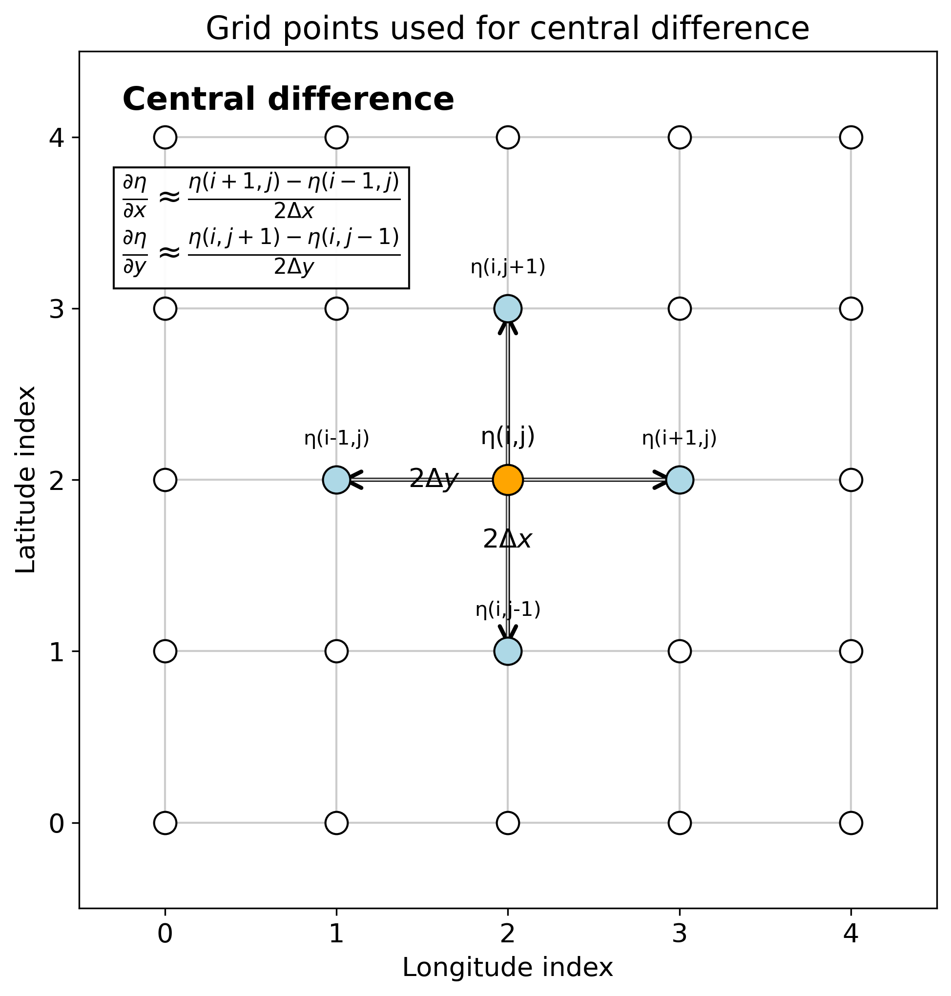
1e-6。中緯度では g/f ≈ 1e5 なので、速度は約 0.1 m/s になります。(η(i+1)-η(i))/dx は、実際には格子点 i ではなく i と i+1 の中間の値です。uとvの位置がずれるため、後で速度勾配を計算するときに扱いが難しくなります。(η(i+1)-η(i-1))/(2dx) は格子点 i 上の勾配として扱えます。したがって、uとvを同じ格子点上で計算できます。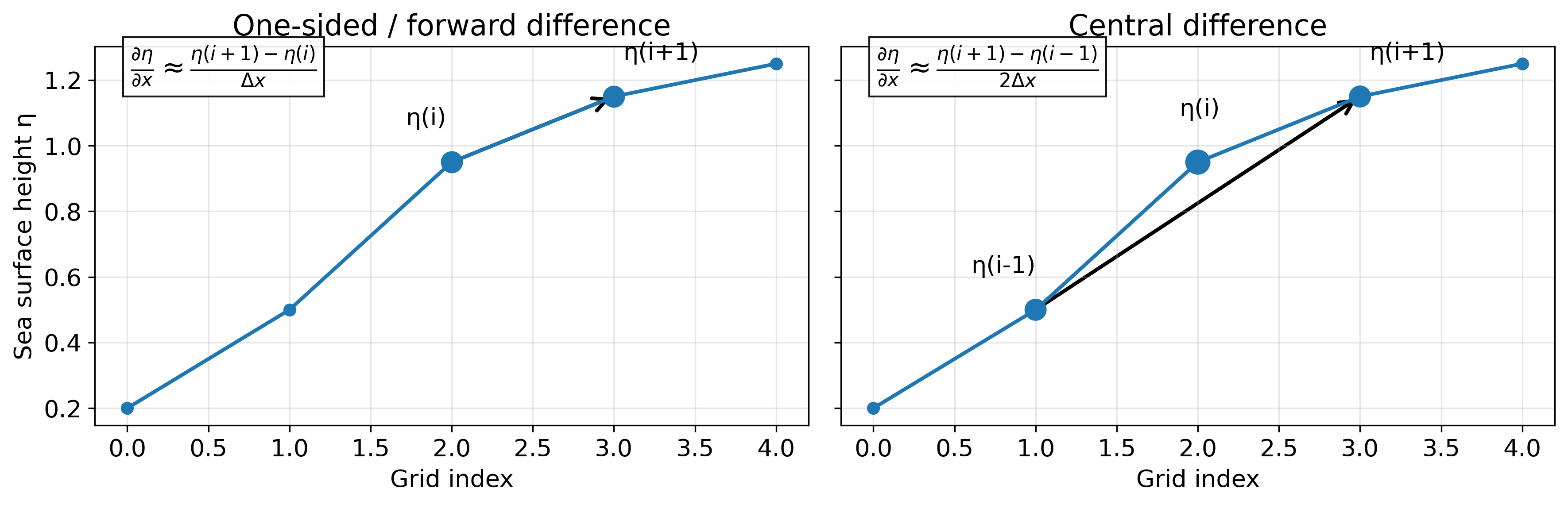
解析用ファイル
以下のNetCDFファイルを、このHTMLファイルと同じフォルダに置いて実行します。MATLABスクリプトは、このページ内のコードをコピーして作成します。NetCDFファイル名は、必要に応じてrun05a冒頭の ncfile を変更してください。
| ファイル | 内容 |
|---|---|
nrt_global_allsat_phy_l4_20240602_20240608.nc | 海面高度データ。longitude, latitude, sla, adt などを含む想定です。 |
run05a_geostrophic_current_central_student.m | 地衡流計算。下の穴埋め版コードをコピーして作成します。 |
run05b_OW_EKE_vorticity_student.m | OW、EKE-like、相対渦度計算。下の穴埋め版コードをコピーして作成します。 |
run05c_SLA_eddy_interpretation_student.m | SLA・ベクトル・OWrotを用いた渦候補の判読。下の穴埋め版コードをコピーして作成します。 |
run05d_closed_contour_eddy_detection_student.m | 閉じたSLAコンターに基づく簡易自動抽出。ページ下部の完全版コードをコピーして作成します。 |
MATLAB基礎関数ミニ辞典
この実習では、数式そのものよりも「MATLABでどう書くか」でつまずきやすいです。以下の関数・記法は、コードを読む前に確認しておきます。
| 関数・記法 | 意味 | この実習での使い方 |
|---|---|---|
deg2rad(x) | degree(度)をradian(ラジアン)に変換します。 | 経度差・緯度差を距離に変換する前に使います。地球半径をかける式では角度をラジアンにする必要があります。 |
sind(x), cosd(x) | 角度をdegreeで与える三角関数です。 | f = 2Ω sin(latitude) や dx = R cos(latitude) Δlon で使います。sin, cos はラジアン用なので混同しないでください。 |
meshgrid | 1次元のlon, latから2次元格子を作ります。 | Lon, Lat を作り、地図上でベクトルやコンターを描くために使います。 |
NaN | Not a Number。計算できない・使わない値を表します。 | 陸、海氷、端の格子、異常値などを計算から除外するために使います。 |
isfinite(A) | A が有限値かどうかをtrue/falseで返します。 | NaNを除いて平均・相関・マスク処理をしたいときに使います。 |
find | 条件を満たすインデックスを取り出します。 | 解析範囲の経度・緯度だけを切り出すときに使います。 |
: | 範囲全体を表します。 | eta(i,:) はi行目の全列、eta(:,j) はj列目の全行です。 |
end | 配列の最後のインデックスです。 | deta_dx(:,end)=NaN は最後の列をNaNにします。 |
conv2 | 2次元畳み込みです。 | このページでは smooth2_nan の中で平滑化に使います。学生が直接穴埋めする対象ではありません。 |
contourc, inpolygon | 等値線を数値として取り出す関数、点が多角形内部にあるか判定する関数です。 | run05dの閉じたSLAコンター検出で使います。発展編なので穴埋めにはしません。 |
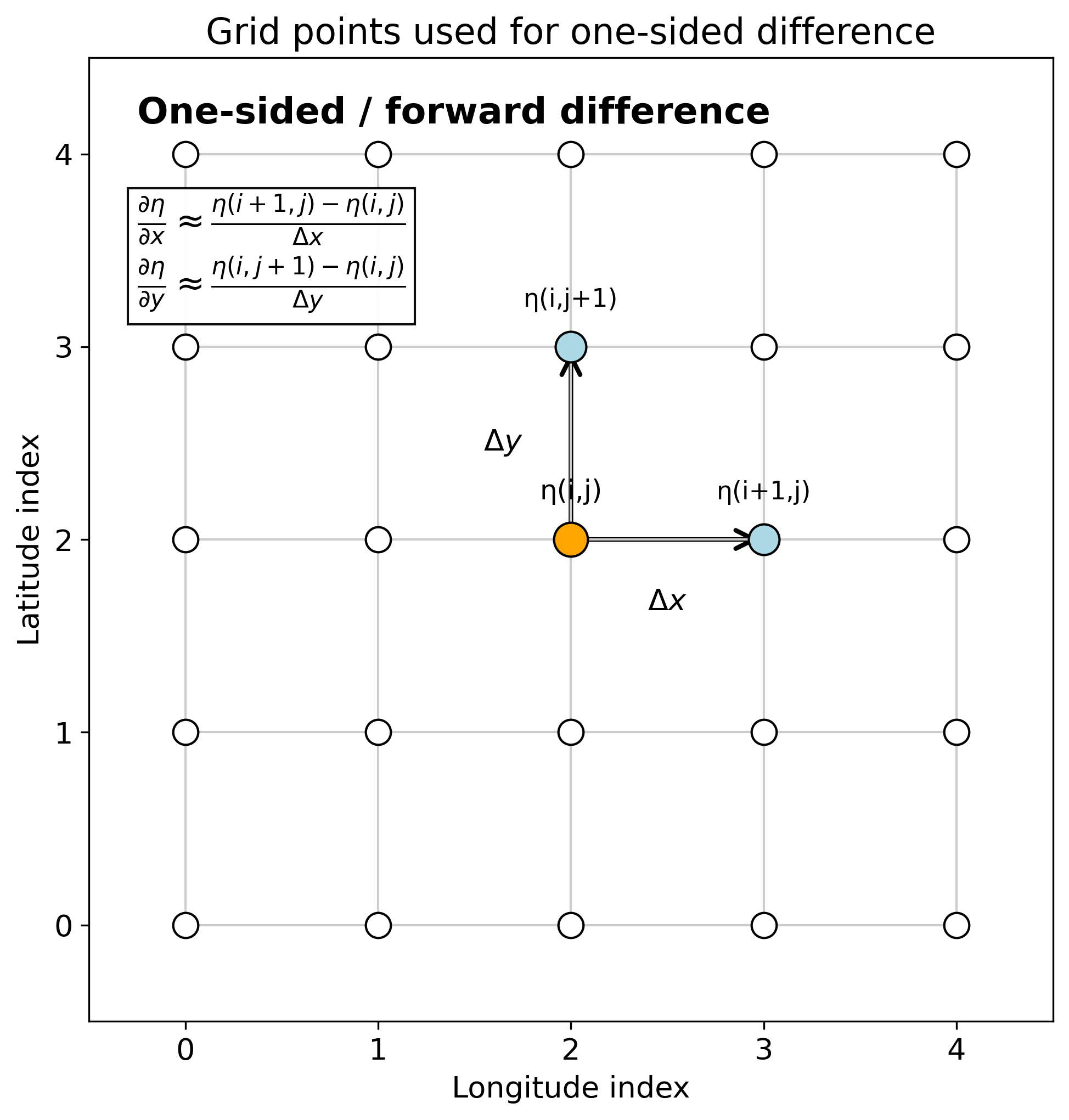
A(i,j) の順に指定します。この実習では、多くの場が [lat lon]、つまり A(i,j) = A(緯度方向, 経度方向) です。i は南北方向、j は東西方向だと考えます。2. 地衡流計算(中央差分):run05a
このスクリプトでは、SLAまたはADTを読み込み、中央差分で dη/dx と dη/dy を求め、地衡流 ug, vg を計算します。穴埋めは、距離換算・差分・地衡流式の本質部分です。
- 経度方向の差
lon(j+1)-lon(j-1)をラジアンに変換する。 - 経度差を距離
dxに変換する。緯度が高いほど東西方向の距離はcos(latitude)倍だけ短くなる。 - 右隣と左隣のSLA差を
dxで割り、dη/dxを求める。 - 同じ考え方で、北隣と南隣のSLA差を
dyで割り、dη/dyを求める。 - 最後に、地衡流の式
u_g=-(g/f)dη/dy,v_g=(g/f)dη/dxをMATLABで書く。
| 数式 | MATLAB変数 | 説明 |
|---|---|---|
| η | eta | SLAまたはADT。 |
| R | Re | 地球半径。ここでは 6371000 m。 |
| Δλ | dlon_rad | 経度差をラジアンに変換したもの。 |
| Δφ | dlat_rad | 緯度差をラジアンに変換したもの。 |
dx = R cos(lat) Δλ | dx | 東西方向の距離。 |
dy = R Δφ | dy | 南北方向の距離。 |
| f = 2Ωsin(lat) | f | コリオリパラメータ。緯度に依存する。 |
deg2rad は「度をラジアンへ変換する関数」です。たとえば、経度差を作るときは lonSub(j+1)-lonSub(j-1) のように、右隣と左隣の差を使います。中央差分では必ず +1 と -1 がペアになります。%% run05a_geostrophic_current_central_student.m
% ============================================================
% Ocean Remote Sensing Practical
% Step 1: Calculate geostrophic current from SLA/ADT
% using central differences
%
% Purpose:
% - Read SLA or ADT from satellite altimetry NetCDF
% - Calculate horizontal gradients on lon-lat grid
% - Calculate geostrophic velocity:
%
% u_g = -(g/f) * d eta / dy
% v_g = (g/f) * d eta / dx
%
% - Save results for the next step
%
% Notes:
% eta = SLA : geostrophic velocity anomaly
% eta = ADT : absolute geostrophic velocity
%
% Required:
% MATLAB only
% ============================================================
clear; close all; clc;
%% ===================== User settings =====================
ncfile = 'nrt_global_allsat_phy_l4_20240602_20240608.nc';
% Display / analysis region
lonlim = [120 170];
latlim = [20 55];
% false: use SLA
% true : use ADT
useAbsolute = false;
% Output directory
outdir = 'run05a_geostrophic_output';
if ~exist(outdir, 'dir')
mkdir(outdir);
end
%% ===================== Constants =====================
g = 9.81; % gravitational acceleration [m s^-2]
Omega = 7.2921159e-5; % Earth's rotation rate [s^-1]
Re = 6371000; % Earth radius [m]
%% ===================== Read data =====================
if ~isfile(ncfile)
error('NetCDF file not found: %s', ncfile);
end
lon = double(ncread(ncfile, 'longitude'));
lat = double(ncread(ncfile, 'latitude'));
ilon = find(lon >= lonlim(1) & lon <= lonlim(2));
ilat = find(lat >= latlim(1) & lat <= latlim(2));
lonSub = lon(ilon);
latSub = lat(ilat);
[Lon, Lat] = meshgrid(lonSub, latSub);
if useAbsolute
etaName = 'adt';
etaLabel = 'ADT';
else
etaName = 'sla';
etaLabel = 'SLA';
end
eta = read_cmems_var_latlon(ncfile, etaName, lon, lat, ilon, ilat);
% Remove ice-covered points if flag_ice exists
try
ice = read_cmems_var_latlon(ncfile, 'flag_ice', lon, lat, ilon, ilat);
eta(ice == 1) = NaN;
catch
end
% Remove unrealistic values
eta(abs(eta) > 5) = NaN;
fprintf('Loaded %s from %s\n', etaName, ncfile);
fprintf('eta size = [%d %d] = [lat lon]\n', size(eta,1), size(eta,2));
%% ===================== Grid spacing =====================
% lon/lat are in degrees.
% Convert degree differences to meter distances.
%
% dx depends on latitude:
% dx = R cos(lat) dlon
%
% dy is almost independent of latitude:
% dy = R dlat
nlat = numel(latSub);
nlon = numel(lonSub);
deta_dx = NaN(nlat, nlon);
deta_dy = NaN(nlat, nlon);
%% ===================== Central difference =====================
% x-direction gradient: d eta / dx
for j = 2:nlon-1
dlon_rad = deg2rad(__________________);
for i = 1:nlat
dx = ________ * cosd(________) * __________;
deta_dx(i,j) = (____________ - ____________) / ____;
end
end
% y-direction gradient: d eta / dy
for i = 2:nlat-1
dlat_rad = deg2rad(__________________);
dy = ________ * __________;
for j = 1:nlon
deta_dy(i,j) = (____________ - ____________) / ____;
end
end
% Edges cannot be calculated by central difference.
% Keep them as NaN.
deta_dx(:,1) = NaN;
deta_dx(:,end) = NaN;
deta_dy(1,:) = NaN;
deta_dy(end,:) = NaN;
%% ===================== Geostrophic current =====================
f = 2 * ________ * sind(_____);
ug = -(____ ./ ____) .* __________;
vg = (____ ./ ____) .* __________;
% Avoid near-equator singularity
ug(abs(f) < 1e-8) = NaN;
vg(abs(f) < 1e-8) = NaN;
speed = sqrt(______.^2 + ______.^2);
% Remove unrealistic speeds
ug(abs(ug) > 5) = NaN;
vg(abs(vg) > 5) = NaN;
speed(abs(speed) > 5) = NaN;
%% ===================== Scaling check =====================
fprintf('\nScaling check:\n');
fprintf(' If eta changes by 0.1 m over 100 km,\n');
fprintf(' slope is about 1e-6.\n');
fprintf(' g/f is about 1e5 at mid-latitudes.\n');
fprintf(' geostrophic speed is about 0.1 m/s.\n');
fprintf('\nComputed geostrophic current:\n');
fprintf(' max |ug| = %.3f m/s\n', max(abs(ug(:)), [], 'omitnan'));
fprintf(' max |vg| = %.3f m/s\n', max(abs(vg(:)), [], 'omitnan'));
fprintf(' max speed = %.3f m/s\n', max(speed(:), [], 'omitnan'));
%% ===================== Figure =====================
figure('Color','w','Position',[100 100 1500 650]);
tiledlayout(1,2,'TileSpacing','compact','Padding','compact');
nexttile;
imagesc(lonSub, latSub, eta);
set(gca,'YDir','normal');
axis tight;
grid on; box on;
colorbar;
caxis([-1 1]);
hold on;
contour(Lon, Lat, eta, -1:0.1:1, 'k', 'LineWidth', 0.4);
title([etaLabel ' and contours']);
xlabel('Longitude');
ylabel('Latitude');
nexttile;
imagesc(lonSub, latSub, speed);
set(gca,'YDir','normal');
axis tight;
grid on; box on;
colorbar;
caxis([0 1.5]);
hold on;
skip = 4;
quiver(Lon(1:skip:end,1:skip:end), Lat(1:skip:end,1:skip:end), ...
ug(1:skip:end,1:skip:end), vg(1:skip:end,1:skip:end), ...
1.5, 'k');
title('Geostrophic speed and vectors from central difference');
xlabel('Longitude');
ylabel('Latitude');
sgtitle('Step 1: Geostrophic current from SLA/ADT using central difference');
exportgraphics(gcf, fullfile(outdir, 'Fig01_geostrophic_current_central.png'), 'Resolution', 180);
%% ===================== Save =====================
outmat = fullfile(outdir, 'geostrophic_current_central.mat');
save(outmat, ...
'ncfile', 'lonSub', 'latSub', 'Lon', 'Lat', ...
'eta', 'etaName', 'etaLabel', ...
'deta_dx', 'deta_dy', ...
'ug', 'vg', 'speed', 'f', ...
'useAbsolute', 'g', 'Omega', 'Re', ...
'-v7.3');
fprintf('\nSaved: %s\n', outmat);
disp('Done.');
%% ===================== Local function =====================
function A = read_cmems_var_latlon(ncfile, varname, lonFull, latFull, ilon, ilat)
raw = ncread(ncfile, varname);
raw = double(squeeze(raw));
info = ncinfo(ncfile, varname);
fillValue = [];
scaleFactor = [];
addOffset = 0;
for ia = 1:numel(info.Attributes)
aname = info.Attributes(ia).Name;
aval = info.Attributes(ia).Value;
if strcmp(aname, '_FillValue')
fillValue = double(aval);
elseif strcmp(aname, 'scale_factor')
scaleFactor = double(aval);
elseif strcmp(aname, 'add_offset')
addOffset = double(aval);
end
end
if ~isempty(fillValue)
raw(raw == fillValue) = NaN;
end
finiteVals = raw(isfinite(raw));
if ~isempty(scaleFactor) && ~isempty(finiteVals)
if prctile(abs(finiteVals), 99) > 50
raw = raw * scaleFactor + addOffset;
end
end
nlon = numel(lonFull);
nlat = numel(latFull);
if size(raw,1) == nlon && size(raw,2) == nlat
Aall = raw.'; % [lat lon]
elseif size(raw,1) == nlat && size(raw,2) == nlon
Aall = raw; % already [lat lon]
else
error('Unexpected size for %s', varname);
end
A = Aall(ilat, ilon);
end
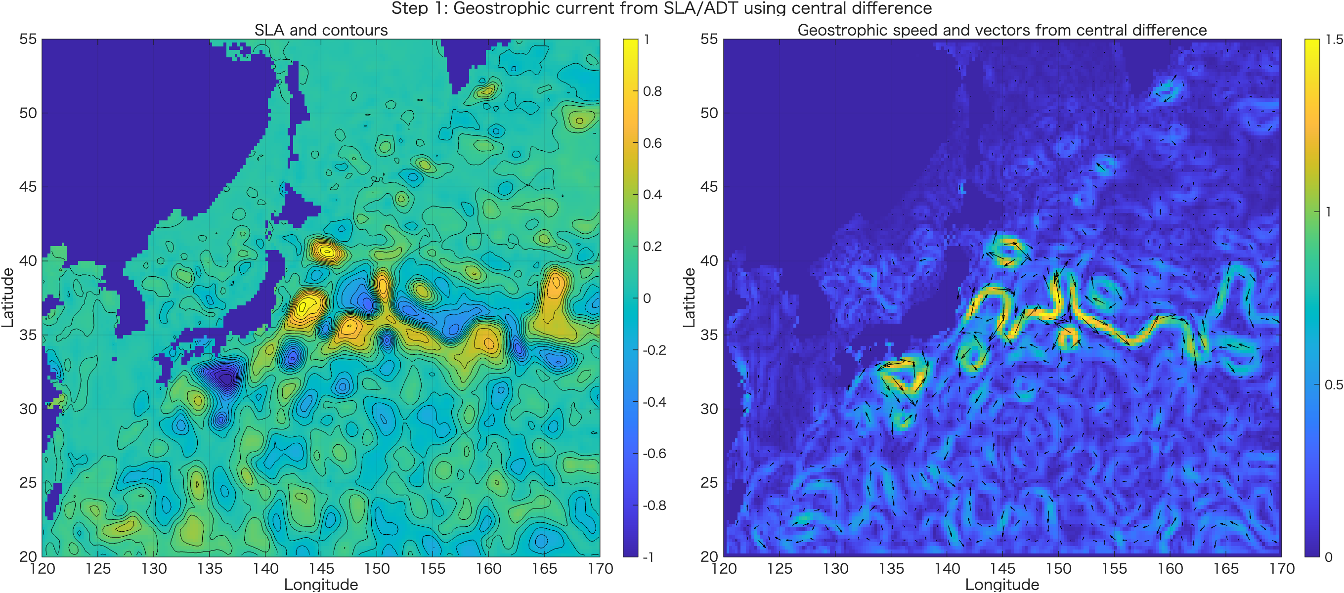
run05aで得られる図
run05aを実行すると、SLA/ADTの空間分布と、それから中央差分で計算した地衡流速・ベクトルが出力されます。SLAの等値線に沿って流れが回り込む様子を確認します。
3. OWパラメータの説明
地衡流 u, v が計算できたら、その空間勾配から相対渦度とひずみを計算します。Okubo-Weissパラメータは、回転とひずみのどちらが卓越しているかを見るための診断量です。
ζ = dv/dx - du/dy流れの回転成分を表します。
ζ/f と規格化すると半球をまたいでも解釈しやすくなります。sn = du/dx - dv/dyss = dv/dx + du/dy流れが引き伸ばされる・せん断される成分です。
OW = strain² - ζ²OW < 0 が回転優勢です。ただし学生には符号が直感的ではありません。OWrot = ζ² - strain²OWrot > 0 が回転優勢です。本実習ではこちらを主に使います。OWrot > 0 は「渦そのもの」ではありません。あくまで回転がひずみより強い領域を示す診断量です。3. OW・EKE-like・相対渦度の計算:run05b
run05aで保存した地衡流を読み込み、速度勾配、相対渦度、ひずみ、OW、OWrot、KE/EKE-likeを計算します。穴埋めは診断量の定義式に集中させています。
- run05aで作った地衡流
ug,vgを読み込む。 - 微分はノイズを増幅するので、速度場を少し平滑化する。この処理は実装上の準備なので穴埋めにはしません。
- 平滑化した速度
ug_s,vg_sからdu/dx,du/dy,dv/dx,dv/dyを計算する。 - 相対渦度
ζ、normal strain、shear strainを定義どおりに組み立てる。 - 回転の強さ
ζ²と、ひずみの強さsn²+ss²を比較する。
| 量 | 式 | MATLABで使う変数 |
|---|---|---|
| 相対渦度 | ζ = dv/dx - du/dy | zeta = dv_dx - du_dy |
| normal strain | sn = du/dx - dv/dy | sn = du_dx - dv_dy |
| shear strain | ss = dv/dx + du/dy | ss = dv_dx + du_dy |
| ひずみの強さ | strain² = sn² + ss² | strain2 |
| 回転の強さ | vorticity² = ζ² | vort2 |
| 通常のOW | OW = strain² - ζ² | OW |
| 授業用OWrot | OWrot = ζ² - strain² | OWrot |
smooth2_nan は自作の平滑化関数です。ここでは「何を平滑化するか」を考えさせるより、OWの定義を理解することを優先するため、スムージング部分は完成コードにしています。%% run05b_OW_EKE_vorticity_student.m
% ============================================================
% Ocean Remote Sensing Practical
% Step 2: Calculate relative vorticity, strain, OWrot, and KE/EKE-like
%
% Input:
% run05a_geostrophic_output/geostrophic_current_central.mat
%
% Output:
% run05b_diagnostics_output/OW_EKE_vorticity.mat
%
% Notes:
% If eta is SLA, ug/vg are geostrophic velocity anomalies.
% Then 0.5*(ug^2+vg^2) can be interpreted as EKE-like.
%
% If eta is ADT, ug/vg are closer to absolute geostrophic velocity.
% Then 0.5*(ug^2+vg^2) is KE, not EKE.
% ============================================================
clear; close all; clc;
%% ===================== Settings =====================
inmat = fullfile('run05a_geostrophic_output', 'geostrophic_current_central.mat');
outdir = 'run05b_diagnostics_output';
if ~exist(outdir, 'dir')
mkdir(outdir);
end
% Smoothing window for velocity before differentiating
% 1 = no smoothing
% 3 or 5 is useful because derivatives amplify noise
smoothWindow = 5;
% Vector skip for plotting
vectorSkip = 4;
%% ===================== Load =====================
if ~isfile(inmat)
error('Input MAT file not found: %s', inmat);
end
S = load(inmat);
lonSub = S.lonSub;
latSub = S.latSub;
Lon = S.Lon;
Lat = S.Lat;
eta = S.eta;
ug = S.ug;
vg = S.vg;
f = S.f;
etaLabel = S.etaLabel;
useAbsolute = S.useAbsolute;
fprintf('Loaded: %s\n', inmat);
fprintf('Field: %s\n', etaLabel);
%% ===================== Smooth velocity =====================
ug_s = smooth2_nan(ug, smoothWindow);
vg_s = smooth2_nan(vg, smoothWindow);
speed = sqrt(______.^2 + ______.^2);
%% ===================== Velocity gradients =====================
[du_dx, du_dy] = central_gradient_lonlat_m(ug_s, lonSub, latSub);
[dv_dx, dv_dy] = central_gradient_lonlat_m(vg_s, lonSub, latSub);
%% ===================== Relative vorticity and strain =====================
% Relative vorticity
zeta = ________ - ________;
% Strain components
sn = ________ - ________; % normal strain
ss = ________ + ________; % shear strain
strain2 = _____.^2 + _____.^2;
vort2 = ______.^2;
% Conventional Okubo-Weiss:
% OW = strain^2 - vorticity^2
% OW < 0 means rotation-dominant.
OW = ________ - ________;
% Teaching-friendly sign:
% OWrot = vorticity^2 - strain^2
% OWrot > 0 means rotation-dominant.
OWrot = ________ - ________;
% Relative vorticity normalized by planetary vorticity
zetaOverF = ______ ./ ____;
zetaOverF(abs(f) < 1e-8) = NaN;
%% ===================== KE / EKE-like =====================
KE = 0.5 * (______.^2 + ______.^2);
if useAbsolute
KElabel = 'Geostrophic KE';
else
KElabel = 'EKE-like from SLA-derived velocity anomaly';
end
%% ===================== Common mask =====================
valid = isfinite(eta) & isfinite(ug_s) & isfinite(vg_s);
speed(~valid) = NaN;
zeta(~valid) = NaN;
zetaOverF(~valid) = NaN;
sn(~valid) = NaN;
ss(~valid) = NaN;
strain2(~valid) = NaN;
vort2(~valid) = NaN;
OW(~valid) = NaN;
OWrot(~valid) = NaN;
KE(~valid) = NaN;
%% ===================== Print summary =====================
fprintf('\nDiagnostics summary:\n');
fprintf(' max speed = %.3f m/s\n', max(speed(:), [], 'omitnan'));
fprintf(' max KE/EKE-like = %.4f m^2/s^2\n', max(KE(:), [], 'omitnan'));
fprintf(' max |zeta/f| = %.3f\n', max(abs(zetaOverF(:)), [], 'omitnan'));
fprintf(' max OWrot = %.3e s^-2\n', max(OWrot(:), [], 'omitnan'));
fprintf(' min OWrot = %.3e s^-2\n', min(OWrot(:), [], 'omitnan'));
%% ===================== Figure =====================
figure('Color','w','Position',[80 80 1500 950]);
tiledlayout(2,2,'TileSpacing','compact','Padding','compact');
nexttile;
imagesc(lonSub, latSub, speed);
set(gca,'YDir','normal');
axis tight; grid on; box on;
colorbar;
caxis([0 1.5]);
hold on;
contour(Lon, Lat, eta, -1:0.1:1, 'k', 'LineWidth', 0.4);
quiver(Lon(1:vectorSkip:end,1:vectorSkip:end), Lat(1:vectorSkip:end,1:vectorSkip:end), ...
ug_s(1:vectorSkip:end,1:vectorSkip:end), vg_s(1:vectorSkip:end,1:vectorSkip:end), ...
1.5, 'k');
title('Geostrophic speed');
xlabel('Longitude'); ylabel('Latitude');
nexttile;
imagesc(lonSub, latSub, KE);
set(gca,'YDir','normal');
axis tight; grid on; box on;
colorbar;
caxis([0 0.3]);
hold on;
contour(Lon, Lat, eta, -1:0.1:1, 'k', 'LineWidth', 0.4);
title(KElabel);
xlabel('Longitude'); ylabel('Latitude');
nexttile;
imagesc(lonSub, latSub, zetaOverF);
set(gca,'YDir','normal');
axis tight; grid on; box on;
colormap(gca, redblue_colormap(256));
colorbar;
caxis([-0.5 0.5]);
hold on;
contour(Lon, Lat, eta, -1:0.1:1, 'k', 'LineWidth', 0.4);
title('Relative vorticity: \zeta / f');
xlabel('Longitude'); ylabel('Latitude');
nexttile;
imagesc(lonSub, latSub, OWrot * 1e10);
set(gca,'YDir','normal');
axis tight; grid on; box on;
colormap(gca, redblue_colormap(256));
colorbar;
caxis([-5 5]);
hold on;
contour(Lon, Lat, eta, -1:0.1:1, 'k', 'LineWidth', 0.4);
contour(Lon, Lat, OWrot, [0 0], 'm', 'LineWidth', 1.0);
title('OW_{rot} = \zeta^2 - strain^2; magenta: OW_{rot}=0');
xlabel('Longitude'); ylabel('Latitude');
sgtitle('Step 2: OW, KE/EKE-like, and relative vorticity');
exportgraphics(gcf, fullfile(outdir, 'Fig01_OW_EKE_vorticity.png'), 'Resolution', 180);
%% ===================== Save =====================
outmat = fullfile(outdir, 'OW_EKE_vorticity.mat');
save(outmat, ...
'lonSub', 'latSub', 'Lon', 'Lat', ...
'eta', 'etaLabel', 'useAbsolute', ...
'ug', 'vg', 'ug_s', 'vg_s', 'speed', ...
'du_dx', 'du_dy', 'dv_dx', 'dv_dy', ...
'zeta', 'zetaOverF', 'sn', 'ss', ...
'strain2', 'vort2', 'OW', 'OWrot', ...
'KE', 'KElabel', 'smoothWindow', ...
'-v7.3');
fprintf('\nSaved: %s\n', outmat);
disp('Done.');
%% ===================== Local functions =====================
function B = smooth2_nan(A, win)
if win <= 1
B = A;
return
end
if mod(win,2) == 0
win = win + 1;
end
K = ones(win, win);
M = isfinite(A);
A0 = A;
A0(~M) = 0;
num = conv2(A0, K, 'same');
den = conv2(double(M), K, 'same');
B = num ./ den;
B(den == 0) = NaN;
end
function [dA_dx, dA_dy] = central_gradient_lonlat_m(A, lon, lat)
Re = 6371000;
nlat = numel(lat);
nlon = numel(lon);
dA_dx = NaN(nlat, nlon);
dA_dy = NaN(nlat, nlon);
for j = 2:nlon-1
dlon_rad = deg2rad(lon(j+1) - lon(j-1));
for i = 1:nlat
dx = Re * cosd(lat(i)) * dlon_rad;
dA_dx(i,j) = (A(i,j+1) - A(i,j-1)) / dx;
end
end
for i = 2:nlat-1
dlat_rad = deg2rad(lat(i+1) - lat(i-1));
dy = Re * dlat_rad;
for j = 1:nlon
dA_dy(i,j) = (A(i+1,j) - A(i-1,j)) / dy;
end
end
end
function cmap = redblue_colormap(n)
if nargin < 1
n = 256;
end
n1 = floor(n/2);
n2 = n - n1;
blue = [linspace(0,1,n1)' linspace(0,1,n1)' ones(n1,1)];
red = [ones(n2,1) linspace(1,0,n2)' linspace(1,0,n2)'];
cmap = [blue; red];
end
run05bで得られる図
run05bでは、地衡流速、KE/EKE-like量、相対渦度 ζ/f、そして OWrot を同じ地図上で比較します。ここで初めて「流れの強さ」と「回転優勢領域」を分けて見られるようになります。
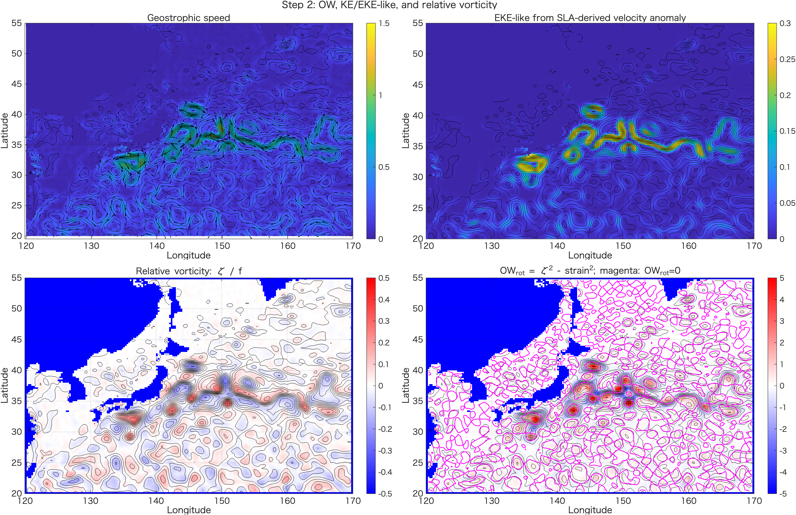
ζ/f、右下が OWrot です。マゼンタ線は OWrot = 0 を示し、その内外で回転優勢・ひずみ優勢が切り替わります。4. 渦の候補:SLA、ベクトル、ζ/f、OWrotを見比べる
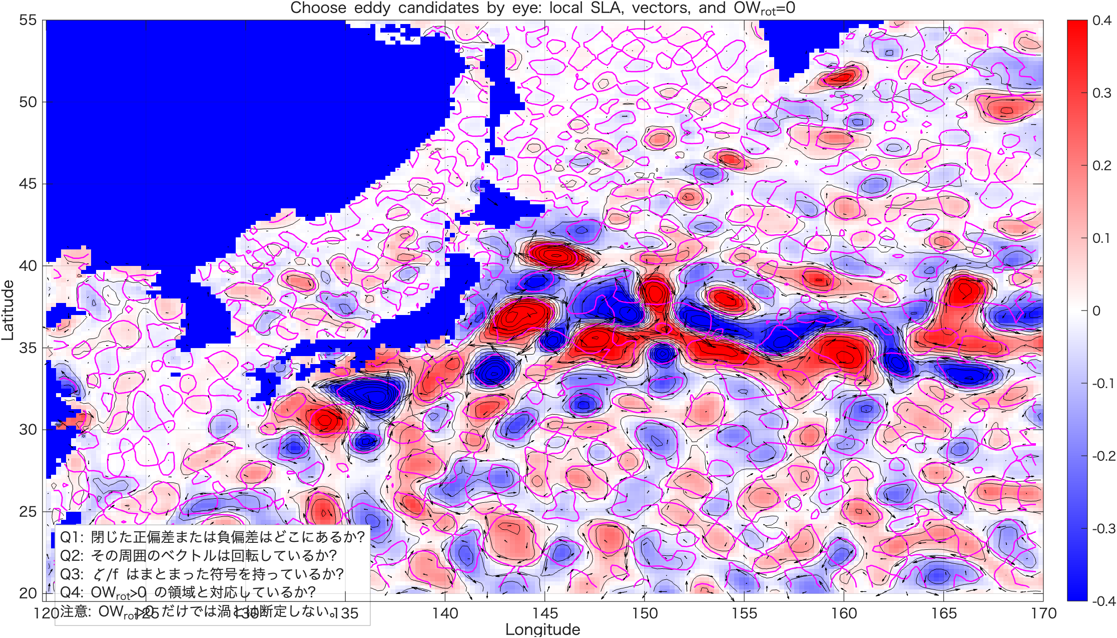
渦らしい構造は、1つの指標だけでは判断しません。SLAの閉じた山・谷、周囲を回る地衡流ベクトル、まとまった相対渦度、そして OWrot > 0 が対応しているかを合わせて確認します。
ζ/f がまとまった正または負のパッチになっているか。OWrot > 0 の回転優勢域と対応するか。4. 渦候補の判読:run05c
このスクリプトは自動検出ではなく、渦候補を人間が判読するための診断図を作ります。候補マスクは「渦かもしれない場所を探す補助」であり、渦検出結果ではありません。
- 大きなスケールのSLA分布を平滑化して、背景場
eta_bgを作る。 - 元のSLAから背景場を引き、局所的なSLA偏差
etaLocalを作る。 - 局所SLA偏差が大きい場所、
|ζ/f|が大きい場所、OWrot>0の場所をそれぞれマスクにする。 - 3つの条件をすべて満たす場所を、渦候補を探す補助マスク
candidateSupportとする。
| 条件 | 意味 | MATLABでの考え方 |
|---|---|---|
| 局所SLA偏差が大きい | 周囲より高い山、または低い谷がある。 | abs(etaLocal) >= localSLA_thr |
| 相対渦度が大きい | 回転成分がある。 | abs(zetaOverF) >= zetaF_thr |
| 回転優勢 | ひずみより回転が強い。 | OWrot > OWrot_thr |
| 候補補助マスク | 3条件をすべて満たす場所。 | 条件1 & 条件2 & 条件3 |
& は「かつ」を表します。つまり A & B & C は、A, B, C のすべてがtrueの場所だけtrueになります。candidateSupport は渦検出結果ではなく、「ここを見に行くと渦らしいかもしれない」という補助図です。%% run05c_SLA_eddy_interpretation_student.m
% ============================================================
% Ocean Remote Sensing Practical
% Step 3: Eddy interpretation using SLA, vectors, zeta/f, OWrot
%
% Input:
% run05b_diagnostics_output/OW_EKE_vorticity.mat
%
% Purpose:
% - Compare SLA/ADT, velocity vectors, relative vorticity, OWrot
% - Identify eddy-like structures by visual interpretation
%
% Important:
% OWrot > 0 does NOT automatically mean "eddy".
% Eddy-like structures should be judged using multiple diagnostics:
%
% 1. closed SLA/ADT anomaly
% 2. rotating velocity vectors
% 3. coherent zeta/f patch
% 4. rotation-dominant OWrot area
%
% ============================================================
clear; close all; clc;
%% ===================== Settings =====================
inmat = fullfile('run05b_diagnostics_output', 'OW_EKE_vorticity.mat');
outdir = 'run05c_eddy_interpretation_output';
if ~exist(outdir, 'dir')
mkdir(outdir);
end
% Local anomaly background smoothing window
bgWindow = 21;
% Vector skip
vectorSkip = 4;
% Candidate support thresholds
% These are not universal. They are only for guided interpretation.
localSLA_thr = 0.05; % m
zetaF_thr = 0.05; % nondimensional
OWrot_thr = 0; % rotation-dominant
%% ===================== Load =====================
if ~isfile(inmat)
error('Input MAT file not found: %s', inmat);
end
S = load(inmat);
lonSub = S.lonSub;
latSub = S.latSub;
Lon = S.Lon;
Lat = S.Lat;
eta = S.eta;
etaLabel = S.etaLabel;
ug_s = S.ug_s;
vg_s = S.vg_s;
speed = S.speed;
zetaOverF = S.zetaOverF;
OWrot = S.OWrot;
KE = S.KE;
KElabel = S.KElabel;
fprintf('Loaded: %s\n', inmat);
fprintf('Field: %s\n', etaLabel);
%% ===================== Local SLA anomaly =====================
% A broad background is removed to emphasize mesoscale structures.
eta_bg = smooth2_nan(eta, bgWindow);
etaLocal = eta - eta_bg;
%% ===================== Candidate support masks =====================
% These masks are not final eddy detection.
% They only indicate places where eddy-like interpretation may be supported.
mask_localSLA = abs(__________) >= _____________;
mask_zeta = abs(__________) >= _________;
mask_OWrot = ________ > _________;
candidateSupport = ______________ & _________ & __________;
% Simple score: how many conditions are satisfied?
eddyScore = double(______________) + double(_________) + double(__________);
eddyScore(~isfinite(etaLocal)) = NaN;
%% ===================== Figure 1: Interpretation panels =====================
figure('Color','w','Position',[80 80 1500 950]);
tiledlayout(2,2,'TileSpacing','compact','Padding','compact');
nexttile;
imagesc(lonSub, latSub, eta);
set(gca,'YDir','normal');
axis tight; grid on; box on;
colorbar;
caxis([-1 1]);
hold on;
contour(Lon, Lat, eta, -1:0.1:1, 'k', 'LineWidth', 0.4);
quiver(Lon(1:vectorSkip:end,1:vectorSkip:end), Lat(1:vectorSkip:end,1:vectorSkip:end), ...
ug_s(1:vectorSkip:end,1:vectorSkip:end), vg_s(1:vectorSkip:end,1:vectorSkip:end), ...
1.5, 'k');
title([etaLabel ' + geostrophic vectors']);
xlabel('Longitude'); ylabel('Latitude');
nexttile;
imagesc(lonSub, latSub, etaLocal);
set(gca,'YDir','normal');
axis tight; grid on; box on;
colormap(gca, redblue_colormap(256));
colorbar;
caxis([-0.4 0.4]);
hold on;
contour(Lon, Lat, eta, -1:0.1:1, 'k', 'LineWidth', 0.4);
title(['Local ' etaLabel ' anomaly']);
xlabel('Longitude'); ylabel('Latitude');
nexttile;
imagesc(lonSub, latSub, zetaOverF);
set(gca,'YDir','normal');
axis tight; grid on; box on;
colormap(gca, redblue_colormap(256));
colorbar;
caxis([-0.5 0.5]);
hold on;
contour(Lon, Lat, eta, -1:0.1:1, 'k', 'LineWidth', 0.4);
title('\zeta / f');
xlabel('Longitude'); ylabel('Latitude');
nexttile;
imagesc(lonSub, latSub, OWrot * 1e10);
set(gca,'YDir','normal');
axis tight; grid on; box on;
colormap(gca, redblue_colormap(256));
colorbar;
caxis([-5 5]);
hold on;
contour(Lon, Lat, eta, -1:0.1:1, 'k', 'LineWidth', 0.4);
contour(Lon, Lat, OWrot, [0 0], 'm', 'LineWidth', 1.0);
title('OW_{rot}; magenta: OW_{rot}=0');
xlabel('Longitude'); ylabel('Latitude');
sgtitle('Step 3: Eddy interpretation using multiple diagnostics');
exportgraphics(gcf, fullfile(outdir, 'Fig01_eddy_interpretation_panels.png'), 'Resolution', 180);
%% ===================== Figure 2: Candidate support =====================
figure('Color','w','Position',[100 100 1500 700]);
tiledlayout(1,2,'TileSpacing','compact','Padding','compact');
nexttile;
imagesc(lonSub, latSub, eddyScore);
set(gca,'YDir','normal');
axis tight; grid on; box on;
colorbar;
caxis([0 3]);
hold on;
contour(Lon, Lat, eta, -1:0.1:1, 'k', 'LineWidth', 0.4);
quiver(Lon(1:vectorSkip:end,1:vectorSkip:end), Lat(1:vectorSkip:end,1:vectorSkip:end), ...
ug_s(1:vectorSkip:end,1:vectorSkip:end), vg_s(1:vectorSkip:end,1:vectorSkip:end), ...
1.5, 'k');
title('Eddy-support score: local SLA + |zeta/f| + OWrot');
xlabel('Longitude'); ylabel('Latitude');
nexttile;
imagesc(lonSub, latSub, double(candidateSupport));
set(gca,'YDir','normal');
axis tight; grid on; box on;
colorbar;
caxis([0 1]);
hold on;
contour(Lon, Lat, eta, -1:0.1:1, 'k', 'LineWidth', 0.4);
quiver(Lon(1:vectorSkip:end,1:vectorSkip:end), Lat(1:vectorSkip:end,1:vectorSkip:end), ...
ug_s(1:vectorSkip:end,1:vectorSkip:end), vg_s(1:vectorSkip:end,1:vectorSkip:end), ...
1.5, 'k');
title('Candidate support mask, not automatic eddy detection');
xlabel('Longitude'); ylabel('Latitude');
sgtitle('Guided eddy interpretation');
exportgraphics(gcf, fullfile(outdir, 'Fig02_candidate_support_mask.png'), 'Resolution', 180);
%% ===================== Figure 3: Guided questions =====================
figure('Color','w','Position',[120 120 1450 760]);
imagesc(lonSub, latSub, etaLocal);
set(gca,'YDir','normal');
axis tight; grid on; box on;
colormap(gca, redblue_colormap(256));
colorbar;
caxis([-0.4 0.4]);
hold on;
contour(Lon, Lat, eta, -1:0.1:1, 'k', 'LineWidth', 0.4);
contour(Lon, Lat, OWrot, [0 0], 'm', 'LineWidth', 1.0);
quiver(Lon(1:vectorSkip:end,1:vectorSkip:end), Lat(1:vectorSkip:end,1:vectorSkip:end), ...
ug_s(1:vectorSkip:end,1:vectorSkip:end), vg_s(1:vectorSkip:end,1:vectorSkip:end), ...
1.5, 'k');
title('Choose eddy candidates by eye: local SLA, vectors, and OW_{rot}=0');
xlabel('Longitude');
ylabel('Latitude');
text(min(lonSub)+0.5, min(latSub)+1.0, { ...
'Q1: 閉じた正偏差または負偏差はどこにあるか?', ...
'Q2: その周囲のベクトルは回転しているか?', ...
'Q3: \zeta/f はまとまった符号を持っているか?', ...
'Q4: OW_{rot}>0 の領域と対応しているか?', ...
'注意: OW_{rot}>0 だけでは渦とは断定しない。'}, ...
'BackgroundColor','w', ...
'EdgeColor',[0.7 0.7 0.7], ...
'FontSize',11);
exportgraphics(gcf, fullfile(outdir, 'Fig03_guided_questions.png'), 'Resolution', 180);
%% ===================== Interpretation guide printed to console =====================
fprintf('\nInterpretation guide:\n');
fprintf(' Eddy-like structure should satisfy several conditions:\n');
fprintf(' 1. closed or nearly closed SLA/ADT anomaly\n');
fprintf(' 2. rotating geostrophic vectors\n');
fprintf(' 3. coherent relative vorticity patch\n');
fprintf(' 4. OWrot > 0, meaning rotation-dominant\n');
fprintf('\n');
fprintf(' Northern Hemisphere sign guide:\n');
fprintf(' positive SLA/ADT anomaly -> anticyclonic tendency -> clockwise rotation\n');
fprintf(' negative SLA/ADT anomaly -> cyclonic tendency -> counterclockwise rotation\n');
fprintf('\n');
fprintf(' OWrot is only a diagnostic, not an eddy detector.\n');
%% ===================== Save =====================
outmat = fullfile(outdir, 'SLA_eddy_interpretation.mat');
save(outmat, ...
'lonSub', 'latSub', 'Lon', 'Lat', ...
'eta', 'etaLocal', 'eta_bg', 'etaLabel', ...
'ug_s', 'vg_s', 'speed', ...
'zetaOverF', 'OWrot', 'KE', 'KElabel', ...
'mask_localSLA', 'mask_zeta', 'mask_OWrot', ...
'candidateSupport', 'eddyScore', ...
'localSLA_thr', 'zetaF_thr', 'OWrot_thr', 'bgWindow', ...
'-v7.3');
fprintf('\nSaved: %s\n', outmat);
disp('Done.');
%% ===================== Local functions =====================
function B = smooth2_nan(A, win)
if win <= 1
B = A;
return
end
if mod(win,2) == 0
win = win + 1;
end
K = ones(win, win);
M = isfinite(A);
A0 = A;
A0(~M) = 0;
num = conv2(A0, K, 'same');
den = conv2(double(M), K, 'same');
B = num ./ den;
B(den == 0) = NaN;
end
function cmap = redblue_colormap(n)
if nargin < 1
n = 256;
end
n1 = floor(n/2);
n2 = n - n1;
blue = [linspace(0,1,n1)' linspace(0,1,n1)' ones(n1,1)];
red = [ones(n2,1) linspace(1,0,n2)' linspace(1,0,n2)'];
cmap = [blue; red];
end
run05cで得られる図
run05cは、自動検出ではなく「判読」のための図を作るスクリプトです。SLA、local SLA anomaly、ζ/f、OWrot を見比べ、渦候補を目で選びます。
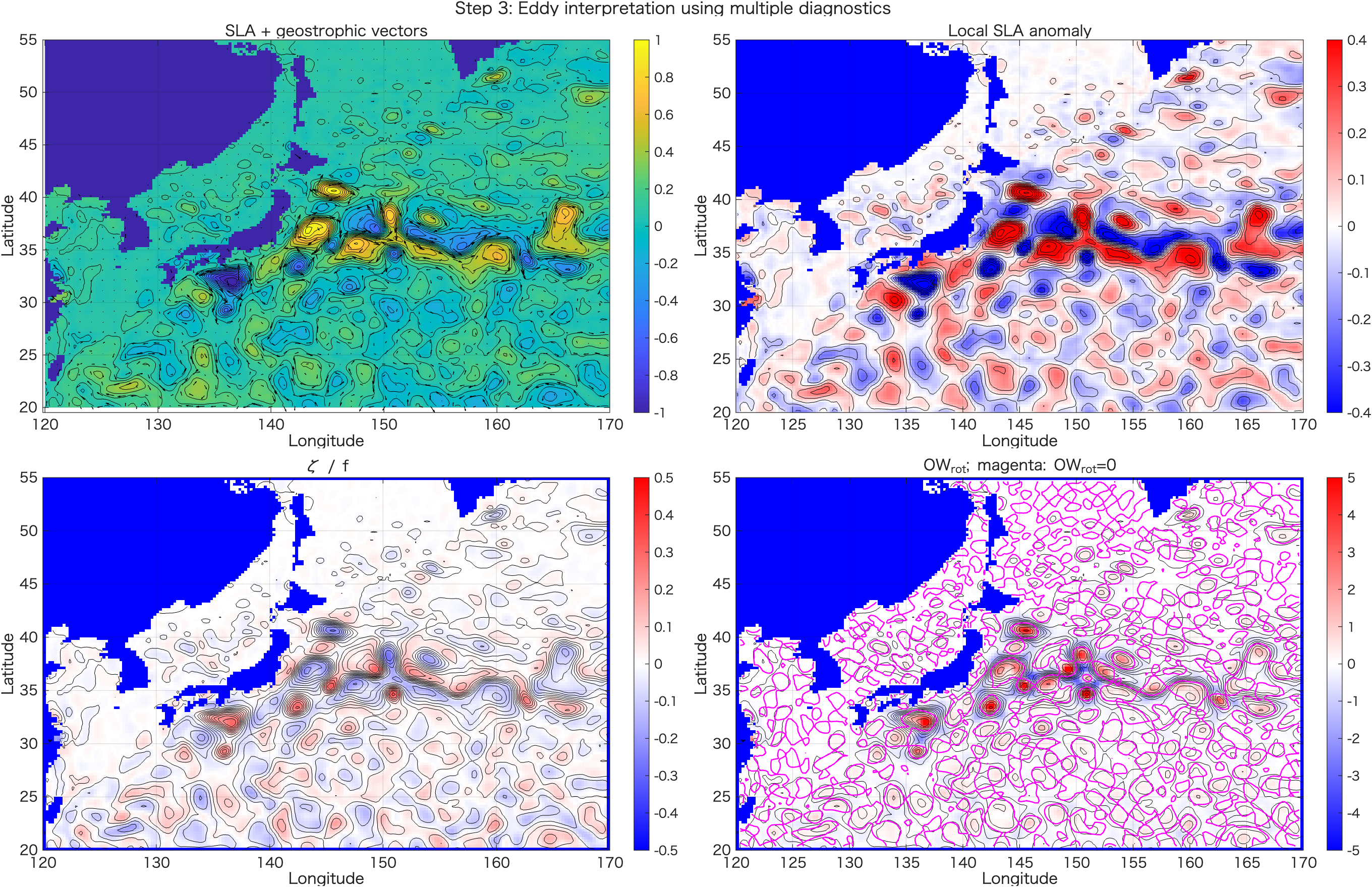
ζ/f、OWrot の比較。単独の指標ではなく、複数の診断量がそろう場所を探します。
OWrot=0 の線を合わせて確認します。5. 渦自動判定アルゴリズム:考え方
ここまでのrun05a〜run05cでは、SLA/ADTから地衡流、相対渦度、OWrotを計算し、人間が図を見て渦候補を判読しました。run05dでは、さらに一歩進んで、閉じたSLA/ADTコンターを使って、渦候補を機械的に抽出する考え方を確認します。
5.1 なぜ閉じたコンターを見るのか
渦は、海面高度場ではしばしば閉じた山または閉じた谷として現れます。SLAまたはADTの等値線が閉じていれば、その内側に局所的な海面高度の高まり、または低まりが存在する可能性があります。
ζ/f や OWrot を使って、閉じたコンター内が本当に回転優勢か確認します。閉じたSLA/ADTコンターを探す → その内側の格子点を取り出す → 面積・半径・重心・SLA極値・振幅・
ζ/f・OWrotを計算する → 入れ子状に重複した候補をまとめる、という流れです。5.2 自動判定の全体フロー
run05dの中では、次の順番で処理します。コードを読むときは、この流れを頭に置いてください。
| 段階 | 何をするか | 対応する主なMATLAB処理 |
|---|---|---|
| 1 | run05bの結果を読み込む | load(inmat) |
| 2 | SLA/ADTを平滑化し、コンター抽出用の場を作る | smooth2_nan |
| 3 | 複数のSLA/ADT等値線を作る | levels = levMin:contourInterval:levMax |
| 4 | 等値線座標を数値として取り出す | contourc |
| 5 | 閉じたコンターだけを残す | 始点と終点の距離を確認 |
| 6 | コンター内の格子点を取り出す | inpolygon |
| 7 | 小さすぎる候補、弱すぎる候補を除外する | minInsidePoints, minAmplitude, minRadius_km |
| 8 | 重心、SLA極値、面積、半径を計算する | mean, max, min, sqrt(area/pi) |
| 9 | ζ/fとOWrotとの整合性を確認する | meanZetaF, owrotFraction |
| 10 | 入れ子コンターの重複をまとめる | duplicateCenterDist_km, haversine_km |
5.3 平滑化:なぜSLA/ADTを少し滑らかにするのか
衛星SLA/ADTには、観測誤差、補間、格子化、細かい前線構造などが含まれます。そのまま細かい等値線を引くと、小さな閉じたコンターが大量に出てしまいます。そこでrun05dでは、コンター抽出の前にSLA/ADTを少し平滑化します。
useSmoothedEta = true;
etaSmoothWindow = 5;

etaForContour = eta;

if useSmoothedEta
    etaForContour = smooth2_nan(eta, etaSmoothWindow);
end
etaSmoothWindow = 5 は、5×5格子程度の近傍平均を使うという意味です。ここで使っている smooth2_nan は自作関数で、NaNを無視しながら周囲の値を平均します。
etaSmoothWindow は大きければよいわけではありません。5.4 コンターレベルを決める
閉じたコンターを探すには、どのSLA/ADT値で等値線を引くかを決める必要があります。run05dでは、SLA/ADTの最小値から最大値まで、0.05 m間隔で等値線を作ります。
contourInterval = 0.05;
contourLevelMin = -1.5;
contourLevelMax =  1.5;

etaMin = min(etaForContour(:), [], 'omitnan');
etaMax = max(etaForContour(:), [], 'omitnan');

levMin = max(contourLevelMin, floor(etaMin / contourInterval) * contourInterval);
levMax = min(contourLevelMax, ceil(etaMax / contourInterval) * contourInterval);

levels = levMin:contourInterval:levMax;
contourInterval = 0.05 は、5 cm刻みで等値線を引くという意味です。細かくすれば候補は増えますが、同じ渦に対して入れ子状のコンターが増えます。粗くすれば候補は減りますが、弱い渦を見落とします。
| パラメータ | 意味 | 値を変えるとどうなるか |
|---|---|---|
contourInterval | 等値線の間隔 | 小さいほど候補が増え、重複も増える |
contourLevelMin | 最低コンターレベル | 極端に低い値を除外できる |
contourLevelMax | 最高コンターレベル | 極端に高い値を除外できる |
5.5 contourc:等値線を「図」ではなく「座標データ」として取り出す
通常の contour は図を描くための関数です。一方、contourc は、等値線の座標を数値配列として取り出します。自動判定では、図を見るだけでなく、コンターの座標を使って内側の格子点を調べたいので contourc を使います。
C = contourc(lonSub, latSub, etaForContour, levels);contourc の出力 C は少し特殊です。ひとつのコンター線ごとに、先頭に「コンターレベル」と「点数」が入り、その後ろにコンターのx座標・y座標が並びます。
C(1,k) = contour level
C(2,k) = number of points
C(:, k+1 : k+npt) = contour coordinates
そのため、run05dでは while ループを使って、C の中からコンター線を1本ずつ取り出します。
k = 1;
while k < size(C,2)

    contourLevel = C(1,k);
    npt = C(2,k);

    x = C(1, k+1:k+npt);
    y = C(2, k+1:k+npt);

    k = k + npt + 1;
end
5.6 閉じたコンターだけを残す
渦境界候補にしたいのは、始点と終点が同じ場所に戻ってくる閉じたコンターです。run05dでは、コンター線の始点と終点の距離を調べ、距離がほぼゼロなら閉じていると判断します。
closeDist_deg = hypot(x(1) - x(end), y(1) - y(end));

if closeDist_deg > 1e-8
    continue;
end
hypot(a,b) は sqrt(a^2 + b^2) を計算するMATLAB関数です。ここでは、始点と終点の経度差・緯度差から距離を計算しています。continue は、条件を満たさない場合にその候補を捨てて次のコンターへ進む、という意味です。
5.7 inpolygon:閉じたコンターの内側を取り出す
閉じたコンターが見つかったら、その内側にある格子点を取り出します。ここで使うのが inpolygon です。
in = inpolygon(Lon, Lat, x, y);
nInside = sum(in(:));
inpolygon は、各格子点 (Lon, Lat) が、多角形 (x, y) の内側にあるかどうかを true/false で返します。in はSLA/ADTと同じサイズのlogical配列になります。
| 変数 | 意味 |
|---|---|
x, y | 閉じたコンター線の座標 |
Lon, Lat | 格子点の経度・緯度 |
in | コンター内ならtrue、外ならfalse |
nInside | コンター内に入った格子点の数 |
コンター内の格子点が少なすぎる場合、その候補は小さすぎて信頼できないので除外します。
if nInside < minInsidePoints
    continue;
end
5.8 振幅:その閉じたコンターの中に山または谷があるか
閉じたコンターがあっても、その内側に十分なSLA/ADTの山や谷がなければ、渦候補としては弱すぎます。そこで、コンター内の最大値・最小値を調べます。
etaInside = etaForContour(in);

etaMaxInside = max(etaInside, [], 'omitnan');
etaMinInside = min(etaInside, [], 'omitnan');

ampPos = etaMaxInside - contourLevel;
ampNeg = contourLevel - etaMinInside;ampPosコンターレベルより内側の最大値がどれだけ高いか。正SLAの山の強さを表します。ampNegコンターレベルより内側の最小値がどれだけ低いか。負SLAの谷の強さを表します。run05dでは、ampPos と ampNeg の大きい方を使って、正SLA候補か負SLA候補かを決めます。また、振幅が minAmplitude = 0.05 m より小さい候補は除外します。
if amplitude < minAmplitude
    continue;
end
5.9 重心とSLA/ADT極値は別物
閉じたコンター内で計算する代表的な位置は2種類あります。ひとつは面積重心、もうひとつはSLA/ADT極値の位置です。この2つは一致するとは限りません。
| 量 | 意味 | run05dの変数 |
|---|---|---|
| 面積重心 | 閉じたコンター領域の幾何学的な中心 | lonCentroid, latCentroid |
| SLA/ADT極値 | コンター内でSLA/ADTが最大または最小になる位置 | lonExtreme, latExtreme |
面積重心は、閉じたコンターの形から決まる中心です。一方、SLA/ADT極値は、山の頂上または谷の底です。渦が非対称な場合、この2つはずれます。
% Area-weighted centroid
wArea = cosd(Lat(in));
lonCentroid = sum(Lon(in) .* wArea, 'omitnan') / sum(wArea, 'omitnan');
latCentroid = sum(Lat(in) .* wArea, 'omitnan') / sum(wArea, 'omitnan');
ここで cosd(Lat) を重みに使っているのは、緯度経度格子では高緯度ほど1度あたりの東西距離が短くなるからです。面積をざっくり補正するために、緯度のcosをかけています。
5.10 面積と半径:渦として大きすぎないか・小さすぎないか
閉じたコンター内の面積を計算し、それを円に換算した半径を求めます。
area_km2 = approximate_area_km2(in, lonSub, latSub, Lon, Lat);
radius_km = sqrt(area_km2 / pi);
ここで使っている考え方は、面積 A をもつ円の半径 r が r = sqrt(A/pi) で表される、というものです。実際の渦は円形とは限りませんが、代表的な大きさを1つの数で表すには便利です。
if radius_km < minRadius_km || radius_km > maxRadius_km
    continue;
end
minRadius_km = 20、maxRadius_km = 300 としているので、半径20 km未満の小さすぎる候補や、300 kmを超える大きすぎる候補は除外されます。
5.11 力学的な整合性:ζ/f と OWrot
閉じたSLA/ADTコンターが見つかっても、それだけでは渦とは断定できません。そこで、コンター内の ζ/f と OWrot を確認します。
zetaFInside = zetaOverF(in);
OWrotInside = OWrot(in);

meanZetaF = mean(zetaFInside, 'omitnan');
owrotFraction = sum(OWrotInside > 0 & isfinite(OWrotInside)) ./ ...
sum(isfinite(OWrotInside));meanZetaFコンター内部の平均的な相対渦度です。符号と大きさから、回転のまとまりを確認します。owrotFractionコンター内部のうち、OWrot > 0 の格子点が占める割合です。回転優勢域がどの程度広がっているかを見ます。run05dでは、これらを使って supportFlag を作っています。ただし、これはあくまで補助判定です。supportFlag = true でも、最終的には図で確認する必要があります。
5.12 最大の難所:入れ子コンターの重複除去
渦の山や谷には、普通、複数の閉じたコンターが入れ子状にできます。たとえば同じ正SLA渦に対して、0.10 m、0.15 m、0.20 m、0.25 m の閉じたコンターがすべて見つかることがあります。これらを全部「別々の渦」と数えると、同じ渦を何度も数えてしまいます。
run05dでは、簡易的に、SLA/ADT極値の位置が近い候補を同じ渦候補グループとしてまとめます。
duplicateCenterDist_km = 50;

if dkm <= duplicateCenterDist_km
    group(end+1) = j;
end
dkm は2つの候補の極値位置の距離です。ここでは、極値が50 km以内にある同じ符号の候補を、同じ渦に属する可能性が高いとみなしています。
同じグループに複数のコンターがある場合、run05dでは代表コンターを1つ選びます。初期設定では、面積が最大のコンターを選びます。
duplicateSelection = "largest_area";これは「同じ渦を囲む入れ子コンターのうち、最も外側に近いものを境界候補にする」という考え方です。
5.13 run05dで調整できる主なパラメータ
自動抽出結果は、設定値に強く依存します。ここを少し変えるだけで、抽出される候補の数や形が変わります。
| パラメータ | 初期値 | 意味 | 大きくすると |
|---|---|---|---|
etaSmoothWindow | 5 | SLA/ADT平滑化窓 | 細かい候補が減るが、小さい渦も消えやすい |
contourInterval | 0.05 m | コンター間隔 | 候補数が減るが、弱いコンターを見落とす |
minInsidePoints | 20 | コンター内の最小格子点数 | 小さい候補が除外されやすくなる |
minAmplitude | 0.05 m | 最小SLA/ADT振幅 | 弱い候補が除外される |
minRadius_km | 20 km | 最小半径 | 小スケール候補が減る |
maxRadius_km | 300 km | 最大半径 | 大きな蛇行も残りやすくなる |
duplicateCenterDist_km | 50 km | 重複判定距離 | 近い候補が同じ渦としてまとめられやすくなる |
5.14 出力図の読み方
run05dでは3つの図を出力します。それぞれの役割は異なります。
| 図 | 見ること |
|---|---|
Fig01_all_raw_closed_contours.png | 抽出されたすべての閉じたコンター。入れ子候補が多いことを確認する図。 |
Fig02_selected_eddy_candidates.png | 重複除去後の代表候補。赤・青の閉コンター、白丸の重心、三角のSLA/ADT極値を見る。 |
Fig03_candidates_on_zetaF_OWrot.png | 自動抽出候補が ζ/f や OWrot と整合しているか確認する図。 |
ζ/f、OWrot がそろっているかを確認します。5. 閉じたSLAコンターによる簡易自動抽出:run05d 完全版
以下は完全スクリプトです。穴埋めではありません。run05a、run05bを先に実行してから、このコードをそのまま実行します。
%% run05d_closed_contour_eddy_detection_student.m
% ============================================================
% Ocean Remote Sensing Practical
% Step 4: Simple closed-contour eddy detection from SLA/ADT
%
% Input:
% run05b_diagnostics_output/OW_EKE_vorticity.mat
%
% Purpose:
% - Extract closed SLA/ADT contours
% - Treat each closed contour as an eddy-region candidate
% - Calculate:
% 1. contour polygon
% 2. area-weighted centroid
% 3. SLA/ADT maximum or minimum inside the contour
% 4. amplitude relative to contour level
% 5. approximate radius
% 6. mean zeta/f
% 7. fraction of OWrot > 0
%
% Important:
% This is a simplified educational version.
% It is NOT the full AVISO / py-eddy-tracker algorithm.
%
% Concept:
% Anticyclonic candidate:
% closed contour surrounding a local SLA/ADT maximum
%
% Cyclonic candidate:
% closed contour surrounding a local SLA/ADT minimum
%
% Eddy centroid:
% area-weighted geometric centroid of grid cells inside contour
%
% Eddy center:
% SLA/ADT maximum or minimum inside contour
%
% ============================================================
clear; close all; clc;
%% ============================================================
% 0. Settings
% ============================================================
inmat = fullfile('run05b_diagnostics_output', 'OW_EKE_vorticity.mat');
outdir = 'run05d_closed_contour_eddy_detection_output';
if ~exist(outdir, 'dir')
mkdir(outdir);
end
% Use smoothed or unsmoothed SLA/ADT for contour detection?
% For noisy fields, smoothing is useful.
useSmoothedEta = true;
% Smoothing window for SLA/ADT before contour extraction.
% Must be odd. 1 means no smoothing.
etaSmoothWindow = 5;
% Contour interval [m].
% Smaller interval gives more contours, but also more duplicate candidates.
contourInterval = 0.05;
% Minimum and maximum contour levels [m].
% These will be clipped by actual data range.
contourLevelMin = -1.5;
contourLevelMax = 1.5;
% Minimum number of grid cells inside a closed contour.
minInsidePoints = 20;
% Minimum eddy amplitude [m].
% amplitude = |SLA extreme - contour level|
minAmplitude = 0.05;
% Approximate eddy radius limits [km].
minRadius_km = 20;
maxRadius_km = 300;
% OWrot support condition.
% This is not mandatory for extraction, but used for diagnostic filtering.
minOWrotFraction = 0.10;
% zeta/f support condition.
% This is not mandatory for extraction, but used for diagnostic filtering.
minAbsMeanZetaF = 0.01;
% Duplicate merging:
% If two candidates have extreme centers closer than this distance,
% they are treated as the same eddy candidate.
duplicateCenterDist_km = 50;
% For each duplicate group, choose:
% "largest_area" or "largest_amplitude"
duplicateSelection = "largest_area";
% Plot settings
vectorSkip = 4;
fprintf('=== run05d: Closed-contour eddy detection ===\n');
fprintf('Input file: %s\n', inmat);
%% ============================================================
% 1. Load diagnostics from run05b
% ============================================================
if ~isfile(inmat)
error('Input MAT file not found: %s', inmat);
end
S = load(inmat);
lonSub = S.lonSub;
latSub = S.latSub;
Lon = S.Lon;
Lat = S.Lat;
eta = S.eta;
etaLabel = S.etaLabel;
ug_s = S.ug_s;
vg_s = S.vg_s;
speed = S.speed;
zetaOverF = S.zetaOverF;
OWrot = S.OWrot;
KE = S.KE;
fprintf('Loaded: %s\n', inmat);
fprintf('etaLabel = %s\n', etaLabel);
fprintf('eta size = [%d %d] = [lat lon]\n', size(eta,1), size(eta,2));
[nlat, nlon] = size(eta);
%% ============================================================
% 2. Prepare SLA/ADT field for contour extraction
% ============================================================
etaForContour = eta;
if useSmoothedEta
etaForContour = smooth2_nan(eta, etaSmoothWindow);
end
% Keep land/invalid mask
etaForContour(~isfinite(eta)) = NaN;
etaMin = min(etaForContour(:), [], 'omitnan');
etaMax = max(etaForContour(:), [], 'omitnan');
levMin = max(contourLevelMin, floor(etaMin / contourInterval) * contourInterval);
levMax = min(contourLevelMax, ceil(etaMax / contourInterval) * contourInterval);
levels = levMin:contourInterval:levMax;
fprintf('\nContour settings:\n');
fprintf(' eta range for contour = %.3f to %.3f m\n', etaMin, etaMax);
fprintf(' contour levels = %.3f to %.3f m, interval %.3f m\n', ...
levMin, levMax, contourInterval);
fprintf(' number of levels = %d\n', numel(levels));
%% ============================================================
% 3. Extract all closed contours
% ============================================================
% contourc requires x vector, y vector, and Z matrix of size [length(y), length(x)].
C = contourc(lonSub, latSub, etaForContour, levels);
allCandidates = struct([]);
icand = 0;
k = 1;
fprintf('\nExtracting closed contours...\n');
while k < size(C,2)
contourLevel = C(1,k);
npt = C(2,k);
x = C(1, k+1:k+npt);
y = C(2, k+1:k+npt);
k = k + npt + 1;
% Need enough points to make a polygon
if npt < 4
continue;
end
% Check if contour is closed
closeDist_deg = hypot(x(1) - x(end), y(1) - y(end));
% Tolerance is small because contourc usually repeats the first point.
if closeDist_deg > 1e-8
continue;
end
% Skip contours touching domain boundary.
% These are often not true closed eddy contours within the domain.
touchesBoundary = any(abs(x - min(lonSub)) < 1e-8) || ...
any(abs(x - max(lonSub)) < 1e-8) || ...
any(abs(y - min(latSub)) < 1e-8) || ...
any(abs(y - max(latSub)) < 1e-8);
if touchesBoundary
continue;
end
% Points inside polygon
in = inpolygon(Lon, Lat, x, y);
nInside = sum(in(:));
if nInside < minInsidePoints
continue;
end
etaInside = etaForContour(in);
if all(~isfinite(etaInside))
continue;
end
% Extreme values inside contour
etaMaxInside = max(etaInside, [], 'omitnan');
etaMinInside = min(etaInside, [], 'omitnan');
ampPos = etaMaxInside - contourLevel;
ampNeg = contourLevel - etaMinInside;
% Decide polarity from which side has larger amplitude.
% polarity = +1 : positive SLA/ADT eddy candidate
% polarity = -1 : negative SLA/ADT eddy candidate
if ampPos >= ampNeg
polarity = +1;
amplitude = ampPos;
tmp = etaForContour;
tmp(~in) = NaN;
[etaExtreme, indExtreme] = max(tmp(:), [], 'omitnan');
else
polarity = -1;
amplitude = ampNeg;
tmp = etaForContour;
tmp(~in) = NaN;
[etaExtreme, indExtreme] = min(tmp(:), [], 'omitnan');
end
if amplitude < minAmplitude
continue;
end
[iyExtreme, ixExtreme] = ind2sub(size(etaForContour), indExtreme);
lonExtreme = Lon(iyExtreme, ixExtreme);
latExtreme = Lat(iyExtreme, ixExtreme);
% Area-weighted centroid.
% On lon-lat grid, approximate grid area weighting by cos(latitude).
wArea = cosd(Lat(in));
lonCentroid = sum(Lon(in) .* wArea, 'omitnan') / sum(wArea, 'omitnan');
latCentroid = sum(Lat(in) .* wArea, 'omitnan') / sum(wArea, 'omitnan');
% Approximate area and radius.
% Estimate grid-cell area from local grid spacing.
area_km2 = approximate_area_km2(in, lonSub, latSub, Lon, Lat);
radius_km = sqrt(area_km2 / pi);
if radius_km < minRadius_km || radius_km > maxRadius_km
continue;
end
% Diagnostics inside contour
zetaFInside = zetaOverF(in);
OWrotInside = OWrot(in);
speedInside = speed(in);
KEInside = KE(in);
meanZetaF = mean(zetaFInside, 'omitnan');
medianZetaF = median(zetaFInside, 'omitnan');
meanSpeed = mean(speedInside, 'omitnan');
maxSpeed = max(speedInside, [], 'omitnan');
meanKE = mean(KEInside, 'omitnan');
owrotFraction = sum(OWrotInside > 0 & isfinite(OWrotInside)) ./ ...
sum(isfinite(OWrotInside));
if isempty(owrotFraction) || isnan(owrotFraction)
owrotFraction = 0;
end
% Dynamical support flag.
% This is diagnostic only.
supportFlag = (owrotFraction >= minOWrotFraction) && ...
(abs(meanZetaF) >= minAbsMeanZetaF);
% Expected zeta/f sign:
% In both hemispheres:
% anticyclonic tendency: zeta/f < 0
% cyclonic tendency : zeta/f > 0
%
% But polarity from SLA sign is not always enough near strong fronts.
if polarity > 0
polarityText = "positive-SLA/ADT candidate";
else
polarityText = "negative-SLA/ADT candidate";
end
icand = icand + 1;
allCandidates(icand).id_raw = icand;
allCandidates(icand).level = contourLevel;
allCandidates(icand).x = x;
allCandidates(icand).y = y;
allCandidates(icand).nContourPoints = npt;
allCandidates(icand).nInside = nInside;
allCandidates(icand).polarity = polarity;
allCandidates(icand).polarityText = polarityText;
allCandidates(icand).amplitude = amplitude;
allCandidates(icand).etaExtreme = etaExtreme;
allCandidates(icand).lonExtreme = lonExtreme;
allCandidates(icand).latExtreme = latExtreme;
allCandidates(icand).ixExtreme = ixExtreme;
allCandidates(icand).iyExtreme = iyExtreme;
allCandidates(icand).lonCentroid = lonCentroid;
allCandidates(icand).latCentroid = latCentroid;
allCandidates(icand).area_km2 = area_km2;
allCandidates(icand).radius_km = radius_km;
allCandidates(icand).meanZetaF = meanZetaF;
allCandidates(icand).medianZetaF = medianZetaF;
allCandidates(icand).owrotFraction = owrotFraction;
allCandidates(icand).meanSpeed = meanSpeed;
allCandidates(icand).maxSpeed = maxSpeed;
allCandidates(icand).meanKE = meanKE;
allCandidates(icand).supportFlag = supportFlag;
end
fprintf(' number of raw closed-contour candidates = %d\n', numel(allCandidates));
if isempty(allCandidates)
warning('No closed-contour eddy candidates found. Try lowering thresholds.');
end
%% ============================================================
% 4. Merge duplicate nested contours
% ============================================================
% Closed contours are often nested around the same SLA maximum/minimum.
% Here we merge candidates whose extreme centers are close to each other.
% Add selection-related fields to all raw candidates first.
% This makes all structures have exactly the same fields.
for q = 1:numel(allCandidates)
allCandidates(q).id = NaN;
allCandidates(q).rawGroup = [];
allCandidates(q).nMerged = 1;
end
% IMPORTANT:
% Initialize selectedCandidates as an empty structure array
% with exactly the same fields as allCandidates.
selectedCandidates = allCandidates([]);
if ~isempty(allCandidates)
nRaw = numel(allCandidates);
used = false(nRaw,1);
isel = 0;
for i = 1:nRaw
if used(i)
continue;
end
lon0 = allCandidates(i).lonExtreme;
lat0 = allCandidates(i).latExtreme;
pol0 = allCandidates(i).polarity;
group = i;
for j = i+1:nRaw
if used(j)
continue;
end
if allCandidates(j).polarity ~= pol0
continue;
end
dkm = haversine_km(lon0, lat0, ...
allCandidates(j).lonExtreme, ...
allCandidates(j).latExtreme);
if dkm <= duplicateCenterDist_km
group(end+1) = j; %#ok<SAGROW>
end
end
used(group) = true;
% Choose representative contour from the group
if duplicateSelection == "largest_amplitude"
amps = arrayfun(@(s) s.amplitude, allCandidates(group));
[~, ibest] = max(amps);
else
areas = arrayfun(@(s) s.area_km2, allCandidates(group));
[~, ibest] = max(areas);
end
bestIndex = group(ibest);
isel = isel + 1;
% IMPORTANT:
% Add the extra fields BEFORE assigning to selectedCandidates.
% Otherwise MATLAB complains about dissimilar structures after
% the first selected candidate.
tmpCandidate = allCandidates(bestIndex);
tmpCandidate.id = isel;
tmpCandidate.rawGroup = group;
tmpCandidate.nMerged = numel(group);
selectedCandidates(isel) = tmpCandidate; %#ok<SAGROW>
end
end
fprintf(' number of selected candidates after merging = %d\n', numel(selectedCandidates));
%% ============================================================
% 5. Create candidate table
% ============================================================
if isempty(selectedCandidates)
T = table();
else
nSel = numel(selectedCandidates);
id = zeros(nSel,1);
polarity = zeros(nSel,1);
level = zeros(nSel,1);
amplitude = zeros(nSel,1);
lonCentroid = zeros(nSel,1);
latCentroid = zeros(nSel,1);
lonExtreme = zeros(nSel,1);
latExtreme = zeros(nSel,1);
etaExtreme = zeros(nSel,1);
area_km2 = zeros(nSel,1);
radius_km = zeros(nSel,1);
meanZetaF = zeros(nSel,1);
owrotFraction = zeros(nSel,1);
meanSpeed = zeros(nSel,1);
maxSpeed = zeros(nSel,1);
supportFlag = false(nSel,1);
nMerged = zeros(nSel,1);
for i = 1:nSel
id(i) = selectedCandidates(i).id;
polarity(i) = selectedCandidates(i).polarity;
level(i) = selectedCandidates(i).level;
amplitude(i) = selectedCandidates(i).amplitude;
lonCentroid(i) = selectedCandidates(i).lonCentroid;
latCentroid(i) = selectedCandidates(i).latCentroid;
lonExtreme(i) = selectedCandidates(i).lonExtreme;
latExtreme(i) = selectedCandidates(i).latExtreme;
etaExtreme(i) = selectedCandidates(i).etaExtreme;
area_km2(i) = selectedCandidates(i).area_km2;
radius_km(i) = selectedCandidates(i).radius_km;
meanZetaF(i) = selectedCandidates(i).meanZetaF;
owrotFraction(i) = selectedCandidates(i).owrotFraction;
meanSpeed(i) = selectedCandidates(i).meanSpeed;
maxSpeed(i) = selectedCandidates(i).maxSpeed;
supportFlag(i) = selectedCandidates(i).supportFlag;
nMerged(i) = selectedCandidates(i).nMerged;
end
T = table(id, polarity, level, amplitude, ...
lonCentroid, latCentroid, lonExtreme, latExtreme, etaExtreme, ...
area_km2, radius_km, meanZetaF, owrotFraction, ...
meanSpeed, maxSpeed, supportFlag, nMerged);
% Sort by amplitude descending
T = sortrows(T, 'amplitude', 'descend');
end
csvFile = fullfile(outdir, 'closed_contour_eddy_candidates.csv');
writetable(T, csvFile);
fprintf('\nSaved candidate table:\n %s\n', csvFile);
%% ============================================================
% 6. Figure: all raw closed contours
% ============================================================
figure('Color','w','Position',[80 80 1500 850]);
imagesc(lonSub, latSub, etaForContour);
set(gca,'YDir','normal');
axis tight; grid on; box on;
colorbar;
caxis([-1 1]);
hold on;
contour(Lon, Lat, etaForContour, levels, 'Color', [0.4 0.4 0.4], 'LineWidth', 0.3);
for i = 1:numel(allCandidates)
if allCandidates(i).polarity > 0
col = [1.0 0.2 0.1]; % red-ish
else
col = [0.1 0.2 1.0]; % blue-ish
end
plot(allCandidates(i).x, allCandidates(i).y, '-', ...
'Color', col, 'LineWidth', 0.8);
end
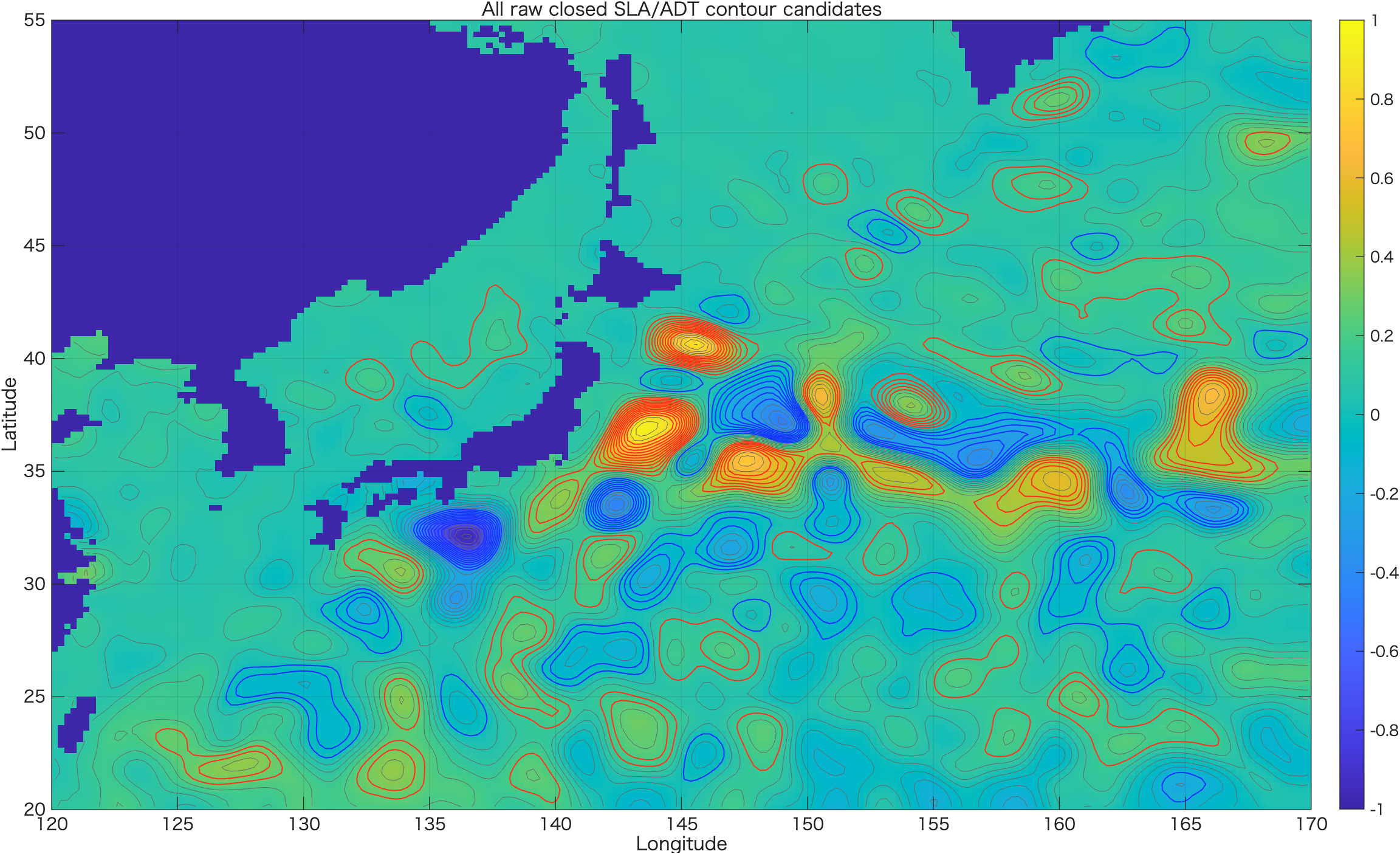
title('All raw closed SLA/ADT contour candidates');
xlabel('Longitude');
ylabel('Latitude');
exportgraphics(gcf, fullfile(outdir, 'Fig01_all_raw_closed_contours.png'), 'Resolution', 180);
%% ============================================================
% 7. Figure: selected eddy candidates
% ============================================================
figure('Color','w','Position',[80 80 1500 900]);
imagesc(lonSub, latSub, etaForContour);
set(gca,'YDir','normal');
axis tight; grid on; box on;
colorbar;
caxis([-1 1]);
hold on;
contour(Lon, Lat, etaForContour, levels, 'Color', [0.55 0.55 0.55], 'LineWidth', 0.25);
% Velocity vectors
quiver(Lon(1:vectorSkip:end,1:vectorSkip:end), ...
Lat(1:vectorSkip:end,1:vectorSkip:end), ...
ug_s(1:vectorSkip:end,1:vectorSkip:end), ...
vg_s(1:vectorSkip:end,1:vectorSkip:end), ...
1.5, 'k');
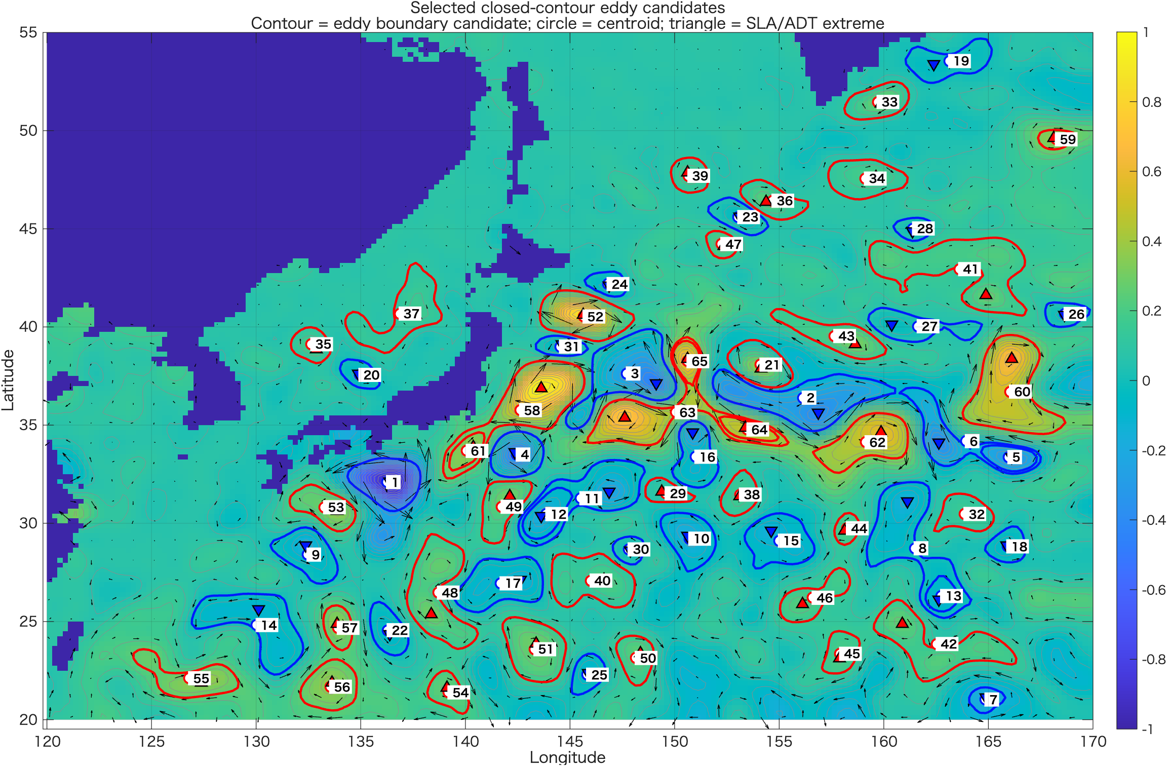
for i = 1:numel(selectedCandidates)
if selectedCandidates(i).polarity > 0
col = [1.0 0.0 0.0];
marker = '^';
else
col = [0.0 0.1 1.0];
marker = 'v';
end
plot(selectedCandidates(i).x, selectedCandidates(i).y, '-', ...
'Color', col, 'LineWidth', 1.8);
% Centroid: circle
plot(selectedCandidates(i).lonCentroid, selectedCandidates(i).latCentroid, ...
'o', 'MarkerSize', 8, ...
'MarkerFaceColor', 'w', ...
'MarkerEdgeColor', col, ...
'LineWidth', 1.5);
% SLA/ADT extreme: triangle
plot(selectedCandidates(i).lonExtreme, selectedCandidates(i).latExtreme, ...
marker, 'MarkerSize', 8, ...
'MarkerFaceColor', col, ...
'MarkerEdgeColor', 'k', ...
'LineWidth', 1.0);
text(selectedCandidates(i).lonCentroid, selectedCandidates(i).latCentroid, ...
sprintf(' %d', i), ...
'Color', 'k', ...
'FontSize', 9, ...
'FontWeight', 'bold', ...
'BackgroundColor', 'w', ...
'Margin', 1);
end
title({'Selected closed-contour eddy candidates', ...
'Contour = eddy boundary candidate; circle = centroid; triangle = SLA/ADT extreme'});
xlabel('Longitude');
ylabel('Latitude');
exportgraphics(gcf, fullfile(outdir, 'Fig02_selected_eddy_candidates.png'), 'Resolution', 180);
%% ============================================================
% 8. Figure: selected candidates over OWrot and zeta/f
% ============================================================
figure('Color','w','Position',[80 80 1500 750]);
tiledlayout(1,2,'TileSpacing','compact','Padding','compact');
nexttile;
imagesc(lonSub, latSub, zetaOverF);
set(gca,'YDir','normal');
axis tight; grid on; box on;
colormap(gca, redblue_colormap(256));
colorbar;
caxis([-0.5 0.5]);
hold on;
contour(Lon, Lat, etaForContour, levels, 'Color', [0.35 0.35 0.35], 'LineWidth', 0.25);
plot_selected_candidates(selectedCandidates);
title('\zeta/f with selected eddy contours');
xlabel('Longitude');
ylabel('Latitude');
nexttile;
imagesc(lonSub, latSub, OWrot * 1e10);
set(gca,'YDir','normal');
axis tight; grid on; box on;
colormap(gca, redblue_colormap(256));
colorbar;
caxis([-5 5]);
hold on;
contour(Lon, Lat, OWrot, [0 0], 'm', 'LineWidth', 0.8);
contour(Lon, Lat, etaForContour, levels, 'Color', [0.35 0.35 0.35], 'LineWidth', 0.25);
plot_selected_candidates(selectedCandidates);
title('OW_{rot} with selected eddy contours');
xlabel('Longitude');
ylabel('Latitude');
sgtitle('Dynamical consistency check for selected closed-contour candidates');
exportgraphics(gcf, fullfile(outdir, 'Fig03_candidates_on_zetaF_OWrot.png'), 'Resolution', 180);
%% ============================================================
% 9. Print interpretation guide
% ============================================================
fprintf('\nInterpretation guide:\n');
fprintf(' Red contours : positive SLA/ADT closed-contour candidates\n');
fprintf(' Blue contours : negative SLA/ADT closed-contour candidates\n');
fprintf(' Circle : area-weighted centroid of the closed contour\n');
fprintf(' Triangle : SLA/ADT maximum or minimum inside the contour\n');
fprintf('\n');
fprintf('Important:\n');
fprintf(' This is not a full AVISO eddy tracker.\n');
fprintf(' It is a simplified closed-contour detector for education.\n');
fprintf(' Check SLA shape, vectors, zeta/f, and OWrot before calling it an eddy.\n');
if ~isempty(T)
fprintf('\nTop 10 candidates by amplitude:\n');
disp(T(1:min(10,height(T)), :));
end
%% ============================================================
% 10. Save MAT file
% ============================================================
outmat = fullfile(outdir, 'closed_contour_eddy_detection.mat');
save(outmat, ...
'lonSub', 'latSub', 'Lon', 'Lat', ...
'eta', 'etaForContour', 'etaLabel', ...
'ug_s', 'vg_s', 'speed', ...
'zetaOverF', 'OWrot', 'KE', ...
'allCandidates', 'selectedCandidates', 'T', ...
'levels', 'contourInterval', ...
'minInsidePoints', 'minAmplitude', ...
'minRadius_km', 'maxRadius_km', ...
'minOWrotFraction', 'minAbsMeanZetaF', ...
'duplicateCenterDist_km', 'duplicateSelection', ...
'useSmoothedEta', 'etaSmoothWindow', ...
'-v7.3');
fprintf('\nSaved MAT file:\n %s\n', outmat);
disp('Done.');
%% ============================================================
% Local functions
% ============================================================
function B = smooth2_nan(A, win)
if win <= 1
B = A;
return
end
if mod(win,2) == 0
win = win + 1;
end
K = ones(win, win);
M = isfinite(A);
A0 = A;
A0(~M) = 0;
num = conv2(A0, K, 'same');
den = conv2(double(M), K, 'same');
B = num ./ den;
B(den == 0) = NaN;
end
function area_km2 = approximate_area_km2(in, lon, lat, Lon, Lat)
Re = 6371000; % m
lon = double(lon(:));
lat = double(lat(:));
if numel(lon) < 2 || numel(lat) < 2
area_km2 = NaN;
return
end
dlon_rad = deg2rad(abs(median(diff(lon), 'omitnan')));
dlat_rad = deg2rad(abs(median(diff(lat), 'omitnan')));
% grid cell area varies with latitude
cellArea_m2 = (Re^2) .* cosd(Lat) .* dlon_rad .* dlat_rad;
cellArea_m2(~in) = NaN;
area_km2 = sum(cellArea_m2(:), 'omitnan') / 1e6;
end
function dkm = haversine_km(lon1, lat1, lon2, lat2)
R = 6371.0; % km
lon1 = deg2rad(lon1);
lat1 = deg2rad(lat1);
lon2 = deg2rad(lon2);
lat2 = deg2rad(lat2);
dlon = lon2 - lon1;
dlat = lat2 - lat1;
a = sin(dlat/2).^2 + cos(lat1).*cos(lat2).*sin(dlon/2).^2;
c = 2 * atan2(sqrt(a), sqrt(1-a));
dkm = R * c;
end
function cmap = redblue_colormap(n)
if nargin < 1
n = 256;
end
n1 = floor(n/2);
n2 = n - n1;
blue = [linspace(0,1,n1)' linspace(0,1,n1)' ones(n1,1)];
red = [ones(n2,1) linspace(1,0,n2)' linspace(1,0,n2)'];
cmap = [blue; red];
end
function plot_selected_candidates(selectedCandidates)
for ii = 1:numel(selectedCandidates)
if selectedCandidates(ii).polarity > 0
col = [1.0 0.0 0.0];
marker = '^';
else
col = [0.0 0.1 1.0];
marker = 'v';
end
plot(selectedCandidates(ii).x, selectedCandidates(ii).y, '-', ...
'Color', col, 'LineWidth', 1.5);
plot(selectedCandidates(ii).lonCentroid, selectedCandidates(ii).latCentroid, ...
'o', 'MarkerSize', 7, ...
'MarkerFaceColor', 'w', ...
'MarkerEdgeColor', col, ...
'LineWidth', 1.2);
plot(selectedCandidates(ii).lonExtreme, selectedCandidates(ii).latExtreme, ...
marker, 'MarkerSize', 7, ...
'MarkerFaceColor', col, ...
'MarkerEdgeColor', 'k', ...
'LineWidth', 0.8);
end
end
run05dで得られる図
run05dは発展編です。閉じたSLA/ADTコンターを抽出し、コンター内の重心、SLA極値、面積、半径などを計算します。自動抽出結果は便利ですが、必ず ζ/f や OWrot と照合して確認します。
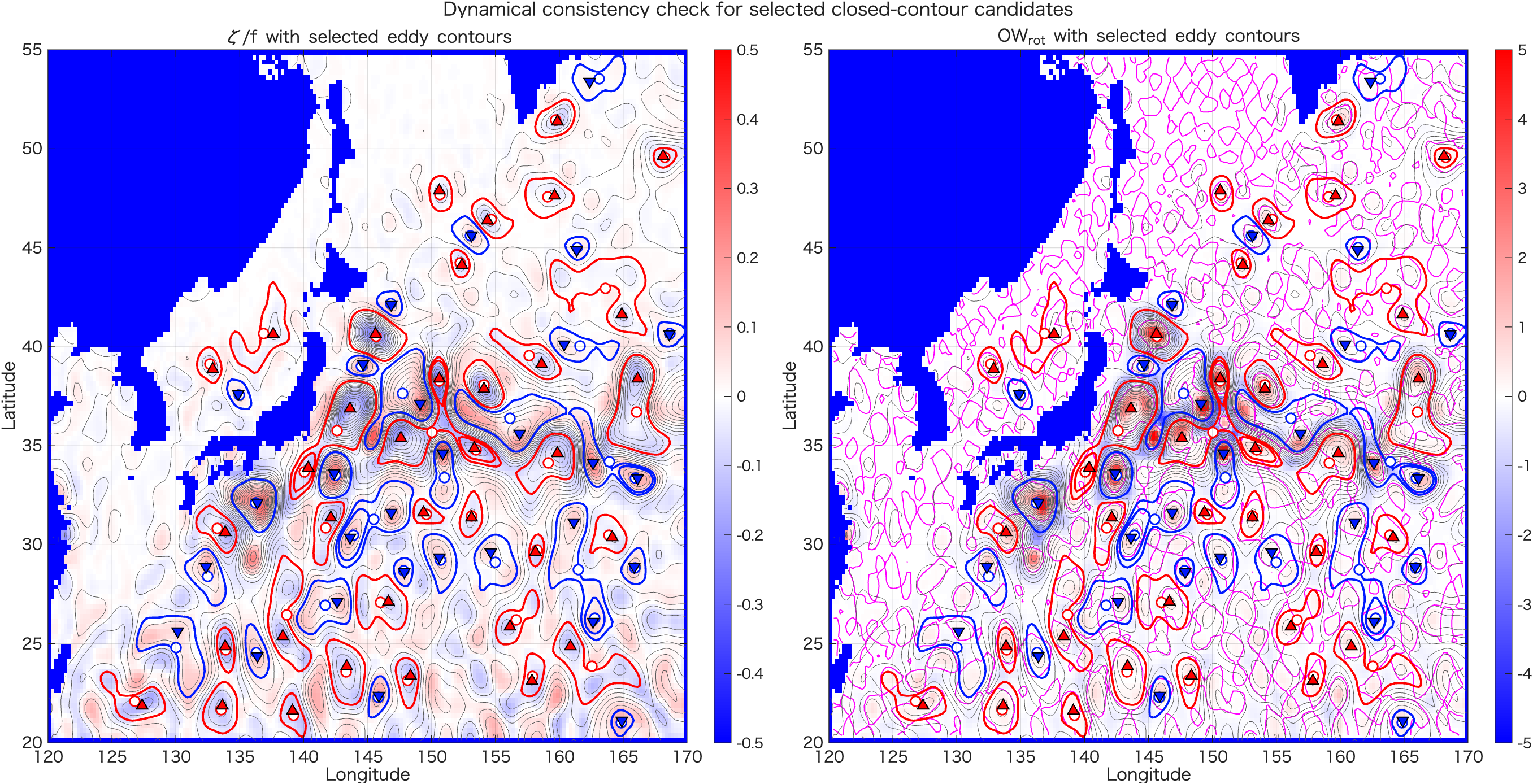
ζ/f と OWrot 上に重ねた確認図。閉じたコンターだけでなく、力学的な整合性も確認します。最後の考察課題
- 前方差分で計算した速度と中央差分で計算した速度では、格子上の位置がどのように異なりますか。
- 10 cm / 100 km 程度のSLA勾配から、どのくらいの地衡流速が期待されますか。
ζ/fは何を表しますか。正負の意味を説明してください。OWrot > 0は何を意味しますか。それだけで渦と呼んでよいですか。- Fig03_guided_questions.pngを見て、渦候補を2つ選び、その根拠をSLA、速度ベクトル、
ζ/f、OWrotの観点から説明してください。 - run05dの自動抽出結果と、自分が目で選んだ渦候補は一致しましたか。一致しない場合、その理由を考えてください。