前節のとおり、データの共分散行列を求め、それに関わる固有値問題を解くことでEOFsを求められることが分かった ここでは、例題に挑戦してみよう。
次に示す、三角関数の線形結合で糞れるデータをEOFsに分けて、第1と第2モードを錘ヲしよう。
データは時間![]() を0から5
を0から5![]() の間、空間では0から
の間、空間では0から![]() の間で取得されるとする。次のような
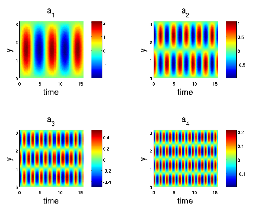
4つの定在波を聞三角関数を想定し、その線形結合を議論する。
の間で取得されるとする。次のような
4つの定在波を聞三角関数を想定し、その線形結合を議論する。
x=0:0.02:pi;
t=0:0.2:5*pi;
[t,x]=meshgrid(t,x);
k=[1 2 3 4];
omega(1)=1;
omega(2)=2;
omega(3)=3;
omega(4)=4;
a(:,:,1)=sin(omega(1).*t-k(1).*(x-pi/2))+sin(omega(1).*t+k(1).*(x-pi/2))+0.1.*rand(size(x));
a(:,:,2)=-0.5.*sin(omega(2).*(t-pi/4)-k(2).*(x-pi/4))-0.5.*sin(omega(2).*(t-pi/4)+k(2).*(x-pi/4))+0.05.*rand(size(x));
a(:,:,3)=0.25.*sin(omega(3).*(t-pi/6)-k(3).*(x-pi/6))+0.25.*sin(omega(3).*(t-pi/6)+k(3).*(x-pi/6))+0.025.*rand(size(x));
a(:,:,4)=-0.1.*sin(omega(4).*(t-pi/8)-k(4).*(x-pi/8))-0.1.*sin(omega(4).*(t-pi/8)+k(4).*(x-pi/8))+0.0125.*rand(size(x));
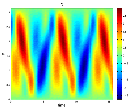
D=sum(a,3);
figure
for i=1:1:4
subplot(2,2,i)
pcolor(t,x,a(:,:,i))
shading flat
colorbar
title(['a_' num2str(i)],'fontsize',15)
xlabel('time','fontsize',15)
ylabel('y','fontsize',15)
end
saveas(gcf,'waves4','png')
print(gcf,'-depsc','waves4')
figure
pcolor(t,x,D);shading flat;colorbar;
title('D','fontsize',15)
xlabel('time','fontsize',15)
ylabel('y','fontsize',15)
saveas(gcf,'sumwaves4','png')
このプログラムを名前をつけて保存して実効してみよう。 以下の様な翠謔ゥける。
次に、データ
![]() の共分散行列
の共分散行列
![]() を求め、
を求め、
![]() の
固有値
の
固有値
![]() と固有ベクトル
と固有ベクトル
![]() を求めよう。固有値問題はMatlabが常備する行列の
計算ツールの内、固有値問題の解法を実行する
を求めよう。固有値問題はMatlabが常備する行列の
計算ツールの内、固有値問題の解法を実行する![]() を用いる。
を用いる。
C=D*D'./size(D,2); % D'はDの転置行列 D*D'./Nは共分散行列
[E,L]=eig(C);
結果として得られた、固有値
![]() と元のデータ
と元のデータ
![]() を用いて、
各モードの振幅
を用いて、
各モードの振幅![]() を求める。具体的には式(15
を求める。具体的には式(15![]() )を実際に計算する。
その後、得られた
)を実際に計算する。
その後、得られた
![]() と固有ベクトル
と固有ベクトル
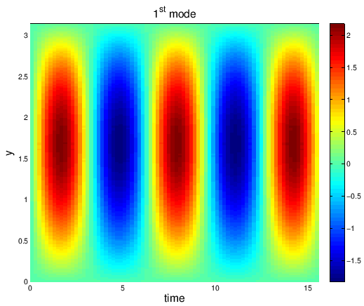
![]() から第1モード
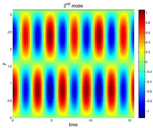
と第2モードの時空間困を抽出する。抽出は、元の式(6
から第1モード
と第2モードの時空間困を抽出する。抽出は、元の式(6![]() )を用いれば良い。
)を用いれば良い。
A=E'*D;
reD1=E(:,end)*A(end,:);
reD2=E(:,end-1)*A(end-1,:);
これで、reD1に第1モード、reD2に第2モードを格納した。 これらを次の様に錘ヲすると以下の様になる。
figure
pcolor(t,x,reD1)
shading flat
colorbar
title('1^{st} mode','fontsize',15)
xlabel('time','fontsize',15)
ylabel('y','fontsize',15)
saveas(gcf,'mode1st','png')
print(gcf,'-depsc','mode1st')
figure
pcolor(t,x,reD2)
shading flat
colorbar
title('2^{nd} mode','fontsize',15)
xlabel('time','fontsize',15)
ylabel('y','fontsize',15)
saveas(gcf,'mode2st','png')
print(gcf,'-depsc','mode2nd')
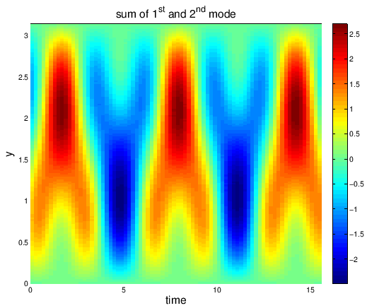
figure
pcolor(t,x,reD1+reD2)
shading flat
colorbar
title('sum of 1^{st} and 2^{nd} mode','fontsize',15)
xlabel('time','fontsize',15)
ylabel('y','fontsize',15)
saveas(gcf,'summode12','png')
print(gcf,'-depsc','summode12')
抽出された第1、2モードの線形結合は、元のデータ