資源環境動態学研究室
English
国立大学法人 東京海洋大学

高野 祥子 (博士研究員)
2002年 東京水産大学(現:東京海洋大学) 卒業
2002年 トルコ共和国エーゲ大学留学
2005年 東京海洋大学大学院 修了
2008-2011年 遠洋水産研究所(現:国際水産資源研究所)
2010年 東京海洋大学大学院 博士号取得
本日の海況の速報値を提供しています。三陸沖合の水温(上図)と塩分(下図)の分布です。水面下180メートル深の分布を表しています。
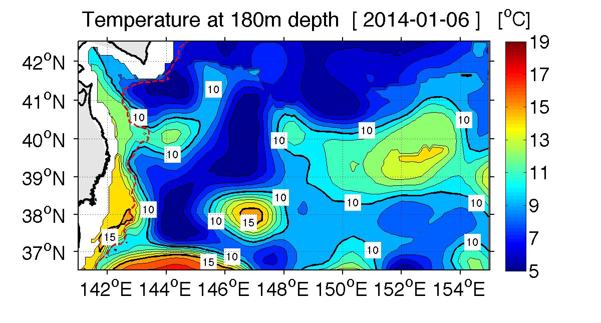
三陸沖海域の水深180mの水温分布図 等値線:1℃毎
* 但し、赤点線より沿岸域の精度は低い可能性があります。
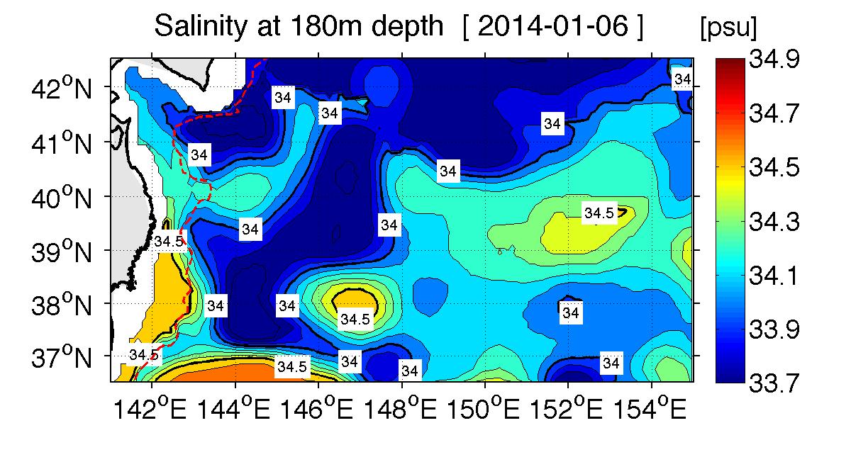
三陸沖海域の水深180mの塩分分布図 等値線:0.1psu毎
* 但し、赤点線より沿岸域の精度は低い可能性があります。
スマートフォン用はこちら
Funded by JST, 復興促進プログラム(A-STEP)
1. Introduction
Near-real time estimation of mesoscale oceanic structures, such as fronts, rings, and streamers that are generated as a result of dynamic current systems, are required for the prediction of the effects of oceanographic processes on climate as well as the location of fertile fishing ground. We will introduce a method for estimating 3-D temperature and salinity structure in near-real time by combining satellite data and in-situ observational data (Argo profiling data). The advantages of this method are that it is simple, low cost (no need for high-performance computing system) and accurate enough to identify mesoscale oceanic structures.
2. Estimation of Isothermal Depth in Two-layer Model
a. Two-layer model
To derive isothermal depth from dynamic topography, we use a simple two-layer model with uniform densities ρ1 and ρ2 for the upper and the lower layers, respectively. Following Goni et al. (1996), the isothermal depths h at a location (x, y) and time t can be equated with the dynamic topography η to give
 (1)
(1)
where ε= (ρ2 -ρ1)/ρ2 is called the measure of stratification (Goni et al. 1996). The variable T is temperature at the interface between the two layers (Fig. 1). The variation of dynamic topography is contributed by the baroclinic component in the first term of Eq. (1), and the second term represents the barotropic pressure component.
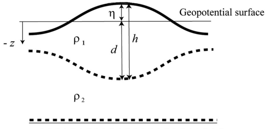
Fig. 1. Schematic of a two-layer model. The thick line indicates the sea surface, and the dashed lines represent two density layers. The geopotential surface is shown by a thin line. In this model, the water column is divided into two layers by a specific temperature T, and η(x, y, t) and d(x, y, t, T) are the surface height and the level of the interface between the layers, respectively, measured from the geopotential surface. The density of the upper layer is ρ1(x, y, t, T) and that of the lower layer is ρ2(x, y, t, T). The thickness of the upper layer is h(x, y, t, T).
b. Empirical thermal model
We propose the following empirical model for the dynamic topography η:
 (2)
(2)
where α’ and β’ are parameters that adjust the ideal two-layer model to a realistic ocean structure and are derived empirically from linear regression analysis for η(x, y, t) and ε(x, y, t, T) h(x, y, t, T). Dynamic topography η(x, y, t) is obtained from satellite altimetry and is an independent parameter. Considering that the dependent random variable h(x, y, t, T) is estimated from η(x, y, t), the modeled equation can be rewritten as
 (3)
(3)
A regular statistical inference can be used for random variable h and independent variable η if we consider ε as a weighting function for h.
c. Data processing and algorithm
Our proposed method requires three datasets: (i) absolute dynamic topography η(x, y, t) acquired by the near-real-time maps of absolute dynamic topography (NRT-MADT) distributed by Archiving, Validation, and Interpretation of Satellite Oceanographic data (AVISO), (ii) ε(xo, yo, to, T) h(xo, yo, to, T) determined from in-situ temperature and salinity Argo profiles, and (iii) ε(x, y, t, T) for the estimation of the isothermal surface in a targeted area obtained from monthly-mean objective analysis of temperature and salinity.
Argo floats provide a measure of the vertical distribution of temperature and salinity between the sea surface and the approximately 2000-m water column every 10 days. Vertical profiles exceeding 1800-m depth were selected within a specified area and time. The data were quality controlled as outlined in Oka et al. (2007) and were interpolated at every 1-m interval from 1 to 1800 m to compute ε h. A depth range was chosen to match the available maximum depth of WOA05. The upper-layer density ρ1 was the average density between the surface and the isotherm depth h, and ρ2 was the average density between h and 1800-m depth.
WOA05 provided data for temperature and salinity from 1- to 1500-m depth at 24 standard depth levels with a 1°horizontal resolution. The data were linearly interpolated to a common grid with the NRT-MADT data.
Figure 2 shows a flowchart for the implementation of the overall method. First, the variables α’ and β’ are derived from linear regression analysis between η(xo, yo, to) and ε(xo, yo, to, T) h(xo, yo, to, T), using the Argo dataset of temperature and salinity, to determine the empirical formula Eq. (3). Confidence intervals at 95% are determined for the estimated depth. Second, ε(x, y, t, T) at the same grid points as for the dynamic topography η(x, y, t) are obtained from WOA05 data instead of from the sparsely distributed Argo data. After having obtained all the necessary parameters for Eq. (3), it is possible to predict the upper-layer depth h(x, y, t, T) at each grid point using the independent variable of dynamic topography (NRT-MADT) η(x, y, t) alone.
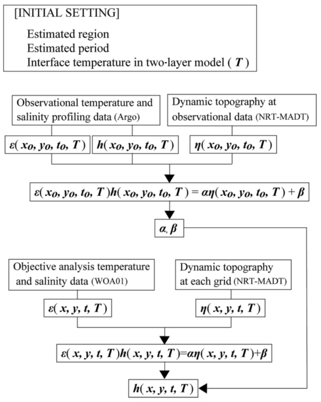
Fig. 2. Flowchart for the method used to estimate three-dimensional thermal structure.
3. Estimation of 3-D Temperature Structure
The 3-D temperature structure was constructed by combining the estimated isothermal depths (as explained in the previous section) with satellite sea surface temperature (SST) and monthly-mean objective analysis of temperature. The value of satellite SST was applied to the surface layer (at 0-m depth) in the 3-D temperature structure. The estimated isothermal depths at some temperature T (e.g. 3, 6, 10 and 15℃) were applied to the mid-layer. The temperature under the estimated isothermal depth at the lowest temperature (e.g. 3℃) was assigned the monthly-mean objective analysis of temperature. Then the values of the temperature (the satellite SST, the estimated temperature and the monthly-mean objective analysis of temperature) at each grid are vertically interpolated into every 1-m interval.
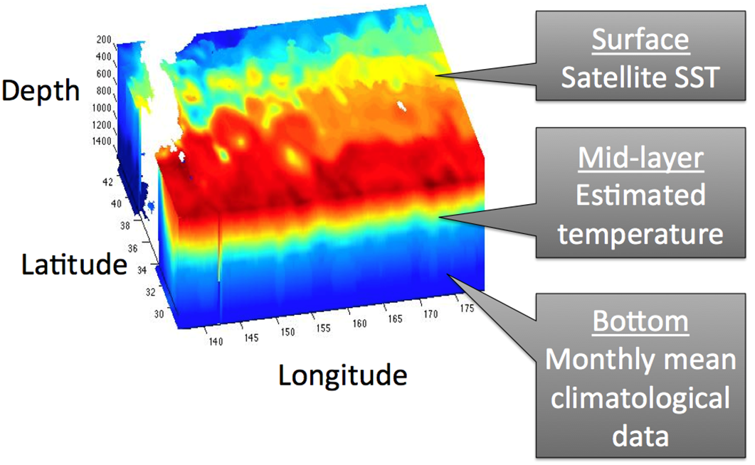
Fig. 3. A image for constructing three-dimensional temperature structure.
4. Estimation of 3-D Salinity Structure
3-D salinity structure is constructed by converting the estimated 3-D temperature to salinity. The conversion model is expressed by calculating a regression analysis between observational data of temperature and salinity from Argo profiling data. The area is divided into blocks by creating 5x5 grid horizontally and 15 layers vertically. The converting model is calculated in each block.
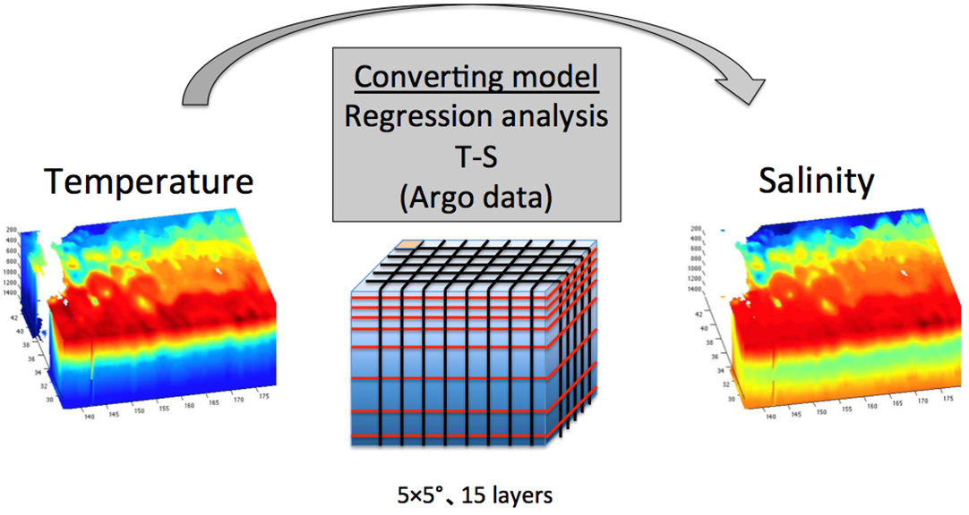
Fig. 4. A image for estimating three dimensional salinity structure.