4. Introduction to NumPy
NumPy is a numerical computation library for Python.
4.1. Overview
NumPy*. - Python provides many useful modules (libraries). - NumPy is a module for numerical computation. - You can load NumPy by import numpy. - As import numpy as np (to read numpy as np), it is common to write np.array() instead of numpy.array(), for example - You can convert a list to a NumPy array with numpy.array(list). - NumPy arrays are equivalent to vectors, matrices, and tensors. - Note that a list and a NumPy array look similar but are different.
matplotlib.pyplot*. - Library for drawing graphs, etc. in Python. - It is common to load import matplotlib.pyplot as plt and name it as plt
Other Frequently Used Libraries
Pandas*.
Pandas is a library for working with two-dimensional tables like Excel
It is common to read
import pandas as pdand name it `pdpd.read_csv()used to read csv files in this course
OpenCV (cv2) - Library with rich functionality for handling images
scikit-learn* - Module for machine learning. It has a full range of functions other than neural networks.
4.2. Generate NumPy array
np.array(list)
[ ]:
# Import NumPy and name it np.
import numpy as np
[ ]:
x = np.array([1,2,3])
print(type(x))
x
<class 'numpy.ndarray'>
array([1, 2, 3])
array.shape is type as array
[ ]:
x.shape
(3,)
where (3,) indicates that it is a 3-dimensional (three-element) vector.
[ ]:
np.zeros(3,) # np.zeros(array type) creates an array with all 0's
array([0., 0., 0.])
matrix of \(A = \begin{bmatrix}1&2&3&4\\2&3&4&5\\3&4&5&6\end{bmatrix}\)
[ ]:
aa = np.array([[1,2,3,4],
               [2,3,4,5],
               [3,4,5,6]])
print(aa.shape)
aa
(3, 4)
array([[1, 2, 3, 4],
       [2, 3, 4, 5],
       [3, 4, 5, 6]])
The way to refer to a value is the same as for a list. The following two lines refer to the same thing.
[ ]:
print(aa[0][1])
aa[0,1]
2
2
Unlike lists, arrays must be rectangular.
[ ]:
a = np.array([[1,2],[3]])
/usr/local/lib/python3.7/dist-packages/ipykernel_launcher.py:1: VisibleDeprecationWarning: Creating an ndarray from ragged nested sequences (which is a list-or-tuple of lists-or-tuples-or ndarrays with different lengths or shapes) is deprecated. If you meant to do this, you must specify 'dtype=object' when creating the ndarray.
  """Entry point for launching an IPython kernel.
4.3. Calculating NumPy arrays
Basically, it is the same as computing a matrix. For example
can be written as follows.
[ ]:
x = np.array([[1,2,3],
              [4,5,6]])
y = np.array([[1,1,1],
              [2,2,2]])

x + y
array([[2, 3, 4],
       [6, 7, 8]])
x * y is a multiplication of the components.
[ ]:
x * y
array([[ 1,  2,  3],
       [ 8, 10, 12]])
Scalar multiplication is performed using 「*」, the same as for ordinary multiplication.
[ ]:
2 * x
array([[ 2,  4,  6],
       [ 8, 10, 12]])
product of matrices
[ ]:
np.dot(x, y.T) # y.T is the transpose of y
array([[ 6, 12],
       [15, 30]])
Unlike what you normally learn in linear algebra, you can also add scalars. The scaler is added to all the components.
[ ]:
x + 2
array([[3, 4, 5],
       [6, 7, 8]])
The feature of applying a function to all elements in this way is called Broadcast.
Broadcast can be used with many NumPy functions in addition to adding scalars. For example, np.sin() applies the sine function to all components.
[ ]:
np.sin(x)
array([[ 0.84147098,  0.90929743,  0.14112001],
       [-0.7568025 , -0.95892427, -0.2794155 ]])
Also, > and == return a boolean value (True = 1, False = 0) for each element, which can also be broadcasted.
[ ]:
print(x>2)
print(x==3)
[[False False  True]
 [ True  True  True]]
[[False False  True]
 [False False False]]
4.4. Statistic
Maximum values
[ ]:
print(x)

# The following two lines both return the maximum value of the array
print(np.max(x))
print(x.max())
[[1 2 3]
 [4 5 6]]
6
6
[ ]:
#maximum value for the 0th index
print(np.max(x, axis =0))

#maximum value for the first index
print(x.max(axis =1))
[4 5 6]
[3 6]
Index that takes the maximum value
[ ]:
print(x.argmax()) # Returns the index of the entire as a first order array.
x.argmax(axis = 0)
5
array([1, 1, 1])
sum
[ ]:
# The following two lines both return the sum of the array components
print(np.sum(x))
print(x.sum())
21
21
[ ]:
# 第0インデックスに関する和
print(np.sum(x, axis =0))

#第1インデックスに関する和
print(x.sum(axis =1))
[5 7 9]
[ 6 15]
Mean, variance, and standard deviation
[ ]:
print( x.mean(axis = 0) )
print( x.var(axis = 0) )
print( x.std(axis = 0) )
[2.5 3.5 4.5]
[2.25 2.25 2.25]
[1.5 1.5 1.5]
4.5. Matplotlib
Matplotlib is a Python library for drawing, and pyplot is a module (i.e., a subset of the library) of Matplotlib for drawing graphs.
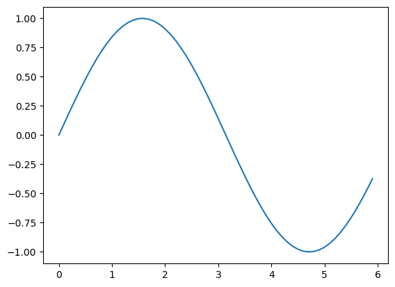
[ ]:
import numpy as np
import matplotlib.pyplot as plt

x = np.arange(0, 6, 0.1) # Generate array of 0.1 increments from 0 to 6
y = np.sin(x) # Broadcast sin() to all components of array x

print('x = ',x)
print('y = ',y)

plt.plot(x,y)

plt.show()# instruction to display (works without, but also displays extra information)
x =  [0.  0.1 0.2 0.3 0.4 0.5 0.6 0.7 0.8 0.9 1.  1.1 1.2 1.3 1.4 1.5 1.6 1.7
 1.8 1.9 2.  2.1 2.2 2.3 2.4 2.5 2.6 2.7 2.8 2.9 3.  3.1 3.2 3.3 3.4 3.5
 3.6 3.7 3.8 3.9 4.  4.1 4.2 4.3 4.4 4.5 4.6 4.7 4.8 4.9 5.  5.1 5.2 5.3
 5.4 5.5 5.6 5.7 5.8 5.9]
y =  [ 0.          0.09983342  0.19866933  0.29552021  0.38941834  0.47942554
  0.56464247  0.64421769  0.71735609  0.78332691  0.84147098  0.89120736
  0.93203909  0.96355819  0.98544973  0.99749499  0.9995736   0.99166481
  0.97384763  0.94630009  0.90929743  0.86320937  0.8084964   0.74570521
  0.67546318  0.59847214  0.51550137  0.42737988  0.33498815  0.23924933
  0.14112001  0.04158066 -0.05837414 -0.15774569 -0.2555411  -0.35078323
 -0.44252044 -0.52983614 -0.61185789 -0.68776616 -0.7568025  -0.81827711
 -0.87157577 -0.91616594 -0.95160207 -0.97753012 -0.993691   -0.99992326
 -0.99616461 -0.98245261 -0.95892427 -0.92581468 -0.88345466 -0.83226744
 -0.77276449 -0.70554033 -0.63126664 -0.55068554 -0.46460218 -0.37387666]
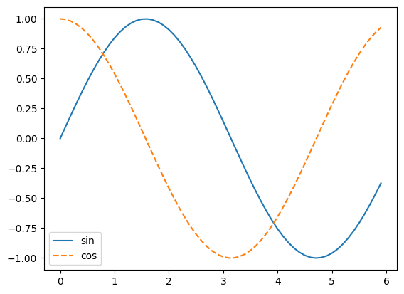
[ ]:
y1 = np.sin(x)
y2 = np.cos(x)

plt.plot(x,y1, label='sin')
plt.plot(x,y2, label='cos', linestyle= '--')
plt.legend() # Display descriptions for graphs

plt.show()