6. Introduction to PyTorch
Notebook (Exercise) for this section (open in another tab)
Video (29 in)
Auto-derivation, model building, and data loading are especially important features of deep learning libraries, not just PyTorch.
Automatic differentiation is a function that calculates the derivative (gradient) of a loss function with respect to input variables or parameters. The data loader creates mini-batches from a dataset for training and evaluation purposes, and transformes the data if necessary. In the case of TensorFlow-Keras, you can train automatically with the fit() method, but in PyTorch you need to create a training function yourself.
Note. * In this notebook, we will not describe the deep learning model itself, because we want to focus on how to use PyTorch.
Specifically, we will not explain the convolutional layer and the pooling layer, which are layers of a neural network that use common weight parameters and relate only pixels that are close to each other to enable efficient learning while suppressing the expressive power of the neural network.
6.1. Automatic differentiation
Let’s look at automatic differentiation using the problem of finding the minimum value of \(z=x^2+ y^2 -2x-4y\) as an example.
Automatic differentiation is implemented by decomposing the operation into simple calculations, creating a 「computation graph,」 and 「back propagating」 the errors (i.e., applying the rules of differentiation of the composite function in the reverse order).
A tool called torchviz is installed to visualize the computation graph.
[ ]:
# Install torchviz, a tool for visualization of computational graphs
!pip install git+https://github.com/szagoruyko/pytorchviz
Collecting git+https://github.com/szagoruyko/pytorchviz
  Cloning https://github.com/szagoruyko/pytorchviz to /tmp/pip-req-build-kub6nsx1
  Running command git clone --filter=blob:none --quiet https://github.com/szagoruyko/pytorchviz /tmp/pip-req-build-kub6nsx1
  Resolved https://github.com/szagoruyko/pytorchviz to commit 0adcd83af8aa7ab36d6afd139cabbd9df598edb7
  Preparing metadata (setup.py) ... done
Requirement already satisfied: torch in /usr/local/lib/python3.10/dist-packages (from torchviz==0.0.2) (2.2.1+cu121)
Requirement already satisfied: graphviz in /usr/local/lib/python3.10/dist-packages (from torchviz==0.0.2) (0.20.1)
Requirement already satisfied: filelock in /usr/local/lib/python3.10/dist-packages (from torch->torchviz==0.0.2) (3.13.1)
Requirement already satisfied: typing-extensions>=4.8.0 in /usr/local/lib/python3.10/dist-packages (from torch->torchviz==0.0.2) (4.10.0)
Requirement already satisfied: sympy in /usr/local/lib/python3.10/dist-packages (from torch->torchviz==0.0.2) (1.12)
Requirement already satisfied: networkx in /usr/local/lib/python3.10/dist-packages (from torch->torchviz==0.0.2) (3.2.1)
Requirement already satisfied: jinja2 in /usr/local/lib/python3.10/dist-packages (from torch->torchviz==0.0.2) (3.1.3)
Requirement already satisfied: fsspec in /usr/local/lib/python3.10/dist-packages (from torch->torchviz==0.0.2) (2023.6.0)
Collecting nvidia-cuda-nvrtc-cu12==12.1.105 (from torch->torchviz==0.0.2)
  Downloading nvidia_cuda_nvrtc_cu12-12.1.105-py3-none-manylinux1_x86_64.whl (23.7 MB)
     ━━━━━━━━━━━━━━━━━━━━━━━━━━━━━━━━━━━━━━━━ 23.7/23.7 MB 27.9 MB/s eta 0:00:00
Collecting nvidia-cuda-runtime-cu12==12.1.105 (from torch->torchviz==0.0.2)
  Downloading nvidia_cuda_runtime_cu12-12.1.105-py3-none-manylinux1_x86_64.whl (823 kB)
     ━━━━━━━━━━━━━━━━━━━━━━━━━━━━━━━━━━━━━━━━ 823.6/823.6 kB 24.7 MB/s eta 0:00:00
Collecting nvidia-cuda-cupti-cu12==12.1.105 (from torch->torchviz==0.0.2)
  Downloading nvidia_cuda_cupti_cu12-12.1.105-py3-none-manylinux1_x86_64.whl (14.1 MB)
     ━━━━━━━━━━━━━━━━━━━━━━━━━━━━━━━━━━━━━━━━ 14.1/14.1 MB 28.0 MB/s eta 0:00:00
Collecting nvidia-cudnn-cu12==8.9.2.26 (from torch->torchviz==0.0.2)
  Downloading nvidia_cudnn_cu12-8.9.2.26-py3-none-manylinux1_x86_64.whl (731.7 MB)
     ━━━━━━━━━━━━━━━━━━━━━━━━━━━━━━━━━━━━━━━━ 731.7/731.7 MB 1.1 MB/s eta 0:00:00
Collecting nvidia-cublas-cu12==12.1.3.1 (from torch->torchviz==0.0.2)
  Downloading nvidia_cublas_cu12-12.1.3.1-py3-none-manylinux1_x86_64.whl (410.6 MB)
     ━━━━━━━━━━━━━━━━━━━━━━━━━━━━━━━━━━━━━━━━ 410.6/410.6 MB 2.0 MB/s eta 0:00:00
WARNING: Retrying (Retry(total=4, connect=None, read=None, redirect=None, status=None)) after connection broken by 'ProtocolError('Connection aborted.', RemoteDisconnected('Remote end closed connection without response'))': /simple/nvidia-cufft-cu12/
Collecting nvidia-cufft-cu12==11.0.2.54 (from torch->torchviz==0.0.2)
  Downloading nvidia_cufft_cu12-11.0.2.54-py3-none-manylinux1_x86_64.whl (121.6 MB)
     ━━━━━━━━━━━━━━━━━━━━━━━━━━━━━━━━━━━━━━━━ 121.6/121.6 MB 8.3 MB/s eta 0:00:00
Collecting nvidia-curand-cu12==10.3.2.106 (from torch->torchviz==0.0.2)
  Downloading nvidia_curand_cu12-10.3.2.106-py3-none-manylinux1_x86_64.whl (56.5 MB)
     ━━━━━━━━━━━━━━━━━━━━━━━━━━━━━━━━━━━━━━━━ 56.5/56.5 MB 10.2 MB/s eta 0:00:00
Collecting nvidia-cusolver-cu12==11.4.5.107 (from torch->torchviz==0.0.2)
  Downloading nvidia_cusolver_cu12-11.4.5.107-py3-none-manylinux1_x86_64.whl (124.2 MB)
     ━━━━━━━━━━━━━━━━━━━━━━━━━━━━━━━━━━━━━━━━ 124.2/124.2 MB 8.3 MB/s eta 0:00:00
Collecting nvidia-cusparse-cu12==12.1.0.106 (from torch->torchviz==0.0.2)
  Downloading nvidia_cusparse_cu12-12.1.0.106-py3-none-manylinux1_x86_64.whl (196.0 MB)
     ━━━━━━━━━━━━━━━━━━━━━━━━━━━━━━━━━━━━━━━━ 196.0/196.0 MB 2.8 MB/s eta 0:00:00
Collecting nvidia-nccl-cu12==2.19.3 (from torch->torchviz==0.0.2)
  Downloading nvidia_nccl_cu12-2.19.3-py3-none-manylinux1_x86_64.whl (166.0 MB)
     ━━━━━━━━━━━━━━━━━━━━━━━━━━━━━━━━━━━━━━━━ 166.0/166.0 MB 7.2 MB/s eta 0:00:00
Collecting nvidia-nvtx-cu12==12.1.105 (from torch->torchviz==0.0.2)
  Downloading nvidia_nvtx_cu12-12.1.105-py3-none-manylinux1_x86_64.whl (99 kB)
     ━━━━━━━━━━━━━━━━━━━━━━━━━━━━━━━━━━━━━━━━ 99.1/99.1 kB 14.1 MB/s eta 0:00:00
Requirement already satisfied: triton==2.2.0 in /usr/local/lib/python3.10/dist-packages (from torch->torchviz==0.0.2) (2.2.0)
Collecting nvidia-nvjitlink-cu12 (from nvidia-cusolver-cu12==11.4.5.107->torch->torchviz==0.0.2)
  Downloading nvidia_nvjitlink_cu12-12.4.99-py3-none-manylinux2014_x86_64.whl (21.1 MB)
     ━━━━━━━━━━━━━━━━━━━━━━━━━━━━━━━━━━━━━━━━ 21.1/21.1 MB 74.1 MB/s eta 0:00:00
Requirement already satisfied: MarkupSafe>=2.0 in /usr/local/lib/python3.10/dist-packages (from jinja2->torch->torchviz==0.0.2) (2.1.5)
Requirement already satisfied: mpmath>=0.19 in /usr/local/lib/python3.10/dist-packages (from sympy->torch->torchviz==0.0.2) (1.3.0)
Building wheels for collected packages: torchviz
  Building wheel for torchviz (setup.py) ... done
  Created wheel for torchviz: filename=torchviz-0.0.2-py3-none-any.whl size=4972 sha256=8d115902d05d931ae4c053d9bd4b2d43ae3470e69a24966f0c4a22b0f176203b
  Stored in directory: /tmp/pip-ephem-wheel-cache-md95rl_u/wheels/44/5a/39/48c1209682afcfc7ad8ae7b3cf7aa0ff08a72e3ac4e5931f1d
Successfully built torchviz
Installing collected packages: nvidia-nvtx-cu12, nvidia-nvjitlink-cu12, nvidia-nccl-cu12, nvidia-curand-cu12, nvidia-cufft-cu12, nvidia-cuda-runtime-cu12, nvidia-cuda-nvrtc-cu12, nvidia-cuda-cupti-cu12, nvidia-cublas-cu12, nvidia-cusparse-cu12, nvidia-cudnn-cu12, nvidia-cusolver-cu12, torchviz
Successfully installed nvidia-cublas-cu12-12.1.3.1 nvidia-cuda-cupti-cu12-12.1.105 nvidia-cuda-nvrtc-cu12-12.1.105 nvidia-cuda-runtime-cu12-12.1.105 nvidia-cudnn-cu12-8.9.2.26 nvidia-cufft-cu12-11.0.2.54 nvidia-curand-cu12-10.3.2.106 nvidia-cusolver-cu12-11.4.5.107 nvidia-cusparse-cu12-12.1.0.106 nvidia-nccl-cu12-2.19.3 nvidia-nvjitlink-cu12-12.4.99 nvidia-nvtx-cu12-12.1.105 torchviz-0.0.2
[ ]:
import torch

# Import a function named make_dot that displays a computation graph from torchviz
from torchviz import make_dot
In Pytorch, all variables are defined as torch.tensor. This corresponds to an array in NumPy. Variables for which you want automatic differentiation (i.e., to be displayed on the graph) should be given the option requires_grad=True.
When you perform a calculation on a tensor, a computation graph is automatically constructed.
The torchviz function make_dot can be used to visualize the graph.
[ ]:
# Create a tensor: scalar (1D) in this case
# Specify as target for automatic differentiation with requires_grad=True
x = torch.tensor(0.0, requires_grad=True)
y = torch.tensor(0.0, requires_grad=True)

# Calculate z
z = (x ** 2 - 2 * x) + (y ** 2 - 4 * y)
print('z:', z)

# Print a graph of the calculation
make_dot(z, params={'x':x,'y':y, 'z':z})
z: tensor(0., grad_fn=<AddBackward0>)

Don’t mind Backward() in the name of the graph label.
Pow means power, Add means add, Sub means subtract, and Mul means multiply.
AccumulatedGrad means to compute the derivative for the variable.
() under a variable indicates the shape of the variable; if it is a scalar, the () is empty.
z.backward() performs automatic differentiation.
Then the partial derivatives
are stored in the variables x.grad and y.grad.
The derivative can be computed by Pytorch only when the variable \(z\) is one-dimensional.
In the case of machine learning, \(z\) is a loss function, so it is 1-dimensional.
[ ]:
# Calculate gradient
z.backward()

# display gradient
print(x.grad)  # dz/dx = 2 x - 2
print(y.grad)  # dz/dy = 2 y - 4
tensor(-2.)
tensor(-4.)
Let’s find the minimum value using the gradient descent method.
Algorithm is as follows.
Determine initial values of \(x\), \(y\) as you like.
Repeat the following steps 2 to 4 a certain number of times.
Compute \(z\).
Calculate the gradients \(\dfrac{\partial z}{\partial x}\) and \(\dfrac{\partial z}{\partial y}\)
For the constant \(\lambda>0\), Update \(x\) and \(y\) as
\[x \leftarrow x - \lambda \frac{\partial z}{\partial x}\]\[y \leftarrow y - \lambda \frac{\partial z}{\partial y}\]where \(\lambda\) in the above equation is called the learning coefficient. Generally, when \(\lambda\) is large, learning is fast but unstable, and when \(\lambda\) is small, learning is slow but stable.
[ ]:
learning_rate = 0.1


# 1. generate initial values with requires_grad=True
x= torch.tensor(0.0, requires_grad=True)
y = torch.tensor(0.0, requires_grad=True)

for i in range(30):
    # 2. calculate z
    z = (x ** 2 - 2 * x) + (y ** 2   - 4 * y)

    # 3. calculate the gradient
    z.backward()

    # Print results :.4f to 4 decimal places
    print(f'i:{i}, x:{x:.4f}, y:{y:.4f}, z:{z:.6f}')

    # 4. Update x and y
    x = x - learning_rate * x.grad
    y = y - learning_rate * y.grad

    # Re-generate x, y before going back to 2: to re-generate the computed graph
    x = x.clone().detach()
    y = y.clone().detach()
    x.requires_grad = True
    y.requires_grad = True
i:0, x:0.0000, y:0.0000, z:0.000000
i:1, x:0.2000, y:0.4000, z:-1.800000
i:2, x:0.3600, y:0.7200, z:-2.952000
i:3, x:0.4880, y:0.9760, z:-3.689280
i:4, x:0.5904, y:1.1808, z:-4.161139
i:5, x:0.6723, y:1.3446, z:-4.463129
i:6, x:0.7379, y:1.4757, z:-4.656403
i:7, x:0.7903, y:1.5806, z:-4.780097
i:8, x:0.8322, y:1.6645, z:-4.859262
i:9, x:0.8658, y:1.7316, z:-4.909928
i:10, x:0.8926, y:1.7853, z:-4.942354
i:11, x:0.9141, y:1.8282, z:-4.963107
i:12, x:0.9313, y:1.8626, z:-4.976388
i:13, x:0.9450, y:1.8900, z:-4.984889
i:14, x:0.9560, y:1.9120, z:-4.990329
i:15, x:0.9648, y:1.9296, z:-4.993810
i:16, x:0.9719, y:1.9437, z:-4.996038
i:17, x:0.9775, y:1.9550, z:-4.997465
i:18, x:0.9820, y:1.9640, z:-4.998377
i:19, x:0.9856, y:1.9712, z:-4.998961
i:20, x:0.9885, y:1.9769, z:-4.999335
i:21, x:0.9908, y:1.9816, z:-4.999575
i:22, x:0.9926, y:1.9852, z:-4.999728
i:23, x:0.9941, y:1.9882, z:-4.999825
i:24, x:0.9953, y:1.9906, z:-4.999888
i:25, x:0.9962, y:1.9924, z:-4.999929
i:26, x:0.9970, y:1.9940, z:-4.999954
i:27, x:0.9976, y:1.9952, z:-4.999971
i:28, x:0.9981, y:1.9961, z:-4.999981
i:29, x:0.9985, y:1.9969, z:-4.999988
When you use an optimizer.
Instead of writing update steps by yourself, you can use the optimizer provided.
[ ]:
import torch.optim as optim

learning_rate = 0.1


# 1. generate initial values with requires_grad=True
x = torch.tensor(0.0, requires_grad=True)
y = torch.tensor(0.0, requires_grad=True)

# Set optimization method Select SGD, Adagrad, Adam, etc.
optimizer = torch.optim.Adam([x,y], lr=learning_rate)

for i in range(30):
    # 2. calculate z
    z = (x ** 2 - 2 * x) + (y ** 2   - 4 * y)

    # 3. calculate the gradient
    z.backward()

    # Print results :.4f to 4 decimal places
    print(f'i:{i}, x:{x:.4f}, y:{y:.4f}, z:{z:.6f}')

    # 4. Update x and y
    optimizer.step()

    # To re-generate the computation graph, optimizer.zero.grad() is performed
    optimizer.zero_grad()
i:0, x:0.0000, y:0.0000, z:0.000000
i:1, x:0.1000, y:0.1000, z:-0.580000
i:2, x:0.1996, y:0.1998, z:-1.118741
i:3, x:0.2984, y:0.2994, z:-1.615657
i:4, x:0.3961, y:0.3985, z:-2.070440
i:5, x:0.4920, y:0.4970, z:-2.483097
i:6, x:0.5858, y:0.5949, z:-2.854013
i:7, x:0.6766, y:0.6918, z:-3.184013
i:8, x:0.7637, y:0.7877, z:-3.474419
i:9, x:0.8464, y:0.8823, z:-3.727085
i:10, x:0.9238, y:0.9754, z:-3.944408
i:11, x:0.9949, y:1.0669, z:-4.129283
i:12, x:1.0589, y:1.1565, z:-4.285008
i:13, x:1.1152, y:1.2440, z:-4.415134
i:14, x:1.1632, y:1.3291, z:-4.523268
i:15, x:1.2024, y:1.4117, z:-4.612880
i:16, x:1.2328, y:1.4914, z:-4.687115
i:17, x:1.2545, y:1.5681, z:-4.748678
i:18, x:1.2677, y:1.6415, z:-4.799774
i:19, x:1.2731, y:1.7114, z:-4.842118
i:20, x:1.2712, y:1.7775, z:-4.876990
i:21, x:1.2627, y:1.8398, z:-4.905329
i:22, x:1.2485, y:1.8980, z:-4.927821
i:23, x:1.2295, y:1.9520, z:-4.945000
i:24, x:1.2066, y:2.0016, z:-4.957319
i:25, x:1.1806, y:2.0467, z:-4.965216
i:26, x:1.1523, y:2.0874, z:-4.969156
i:27, x:1.1227, y:2.1236, z:-4.969660
i:28, x:1.0926, y:2.1553, z:-4.967309
i:29, x:1.0628, y:2.1825, z:-4.962748
6.2. How to use the Datase and Dataloader
Next, let’s look at how to use Dataset and Dataloader with a dataset for 37 different image classification problems of cats and dogs.
Dataset is a class for processing data and calling it in slice notation, and Dataloader is a class for extracting mini-batches (subsets of data) from Dataset.
I think these two are the most confusing parts of PyTorch. (TensorFlow-Keras has a similar function, but it is a bit easier to understand.)
Download Data.
The original data is available at http://www.robots.ox.ac.uk/~vgg/data/pets/ under CC-BY(Attribution)-SA(Inheritance) license. This time, we will distribute it with the following directory structure from Dropbox. This is also licensed under CC-BY-SA. This is also licensed under CC-BY-SA.
pet_dataset/
    train/
        name of species 1/
            x1_1.jpg
            x1_2.jpg
            x1_3.jpg
            ...
        name of species 2/
            x2_2.jpg
            x2_3.jpg
            ...
    val/
        name of species 1/
            x1_1.jpg
            x1_2.jpg
            ...
        name of species 2/
            x2_1.jpg
            x2_2.jpg
            ...
[ ]:
# download with wget -O filename is an option specifying the name of the file to save
!wget 'https://www.dropbox.com/s/6zhb4wm7u6fqs8r/pet_dataset.zip?dl=0' -O pet_dataset.zip

# Unzip the zip file: -q is an option to stop displaying the output
!unzip -q pet_dataset.zip
--2024-03-14 02:36:19--  https://www.dropbox.com/s/6zhb4wm7u6fqs8r/pet_dataset.zip?dl=0
Resolving www.dropbox.com (www.dropbox.com)... 162.125.5.18, 2620:100:601d:18::a27d:512
Connecting to www.dropbox.com (www.dropbox.com)|162.125.5.18|:443... connected.
HTTP request sent, awaiting response... 302 Found
Location: /s/raw/6zhb4wm7u6fqs8r/pet_dataset.zip [following]
--2024-03-14 02:36:19--  https://www.dropbox.com/s/raw/6zhb4wm7u6fqs8r/pet_dataset.zip
Reusing existing connection to www.dropbox.com:443.
HTTP request sent, awaiting response... 302 Found
Location: https://uc1b5436d551d96d9715a2156dc9.dl.dropboxusercontent.com/cd/0/inline/CPA8KWrLwJ9Aj8rEE5wxXVaiGtLr2d_2mW-1OsLjhJ2dNmx-eJAtOm21jtrg9AEbz0VfLXTY8DRhEq6qz_kkafut39JQcgq6Np-mKYdazxCOJeZO7Oth5XClPe7nTRR9GgU/file# [following]
--2024-03-14 02:36:19--  https://uc1b5436d551d96d9715a2156dc9.dl.dropboxusercontent.com/cd/0/inline/CPA8KWrLwJ9Aj8rEE5wxXVaiGtLr2d_2mW-1OsLjhJ2dNmx-eJAtOm21jtrg9AEbz0VfLXTY8DRhEq6qz_kkafut39JQcgq6Np-mKYdazxCOJeZO7Oth5XClPe7nTRR9GgU/file
Resolving uc1b5436d551d96d9715a2156dc9.dl.dropboxusercontent.com (uc1b5436d551d96d9715a2156dc9.dl.dropboxusercontent.com)... 162.125.5.15, 2620:100:601d:15::a27d:50f
Connecting to uc1b5436d551d96d9715a2156dc9.dl.dropboxusercontent.com (uc1b5436d551d96d9715a2156dc9.dl.dropboxusercontent.com)|162.125.5.15|:443... connected.
HTTP request sent, awaiting response... 302 Found
Location: /cd/0/inline2/CPD6YWa9virdyjQ6f3ivAcUx5d8oQWU6xRL-iyvfOOGhfBrSrCl2CJVAG20IaM4PBlTpRkTorZ9j2KAhgCWEyz6QMsHnx16kJ1qZe7lfaF11WWQJ1Nc8EwHmCghGNp_UhlNdkBVoe4bHgO5MtVURWF5LmeGC5_LVaJJG41ihNf_TQUiTQuoV2Nj-dqH5yuxirnAqYQ1_t3IyJ29TluS6_pXUVcV1tKnp9eDT4DgNFhbZK-LSOsw3dB7KxzXpYC407iHF68f6-iC6sKKLJX8sb4xXMX2sM-1UCPuRLiTQPUPPOmQ6UxfC1N9ITYuj1LuvBidhAGV0IbQml7tLCsq0aCjgCNpF8FArX7e9s_0_6iudtQ/file [following]
--2024-03-14 02:36:20--  https://uc1b5436d551d96d9715a2156dc9.dl.dropboxusercontent.com/cd/0/inline2/CPD6YWa9virdyjQ6f3ivAcUx5d8oQWU6xRL-iyvfOOGhfBrSrCl2CJVAG20IaM4PBlTpRkTorZ9j2KAhgCWEyz6QMsHnx16kJ1qZe7lfaF11WWQJ1Nc8EwHmCghGNp_UhlNdkBVoe4bHgO5MtVURWF5LmeGC5_LVaJJG41ihNf_TQUiTQuoV2Nj-dqH5yuxirnAqYQ1_t3IyJ29TluS6_pXUVcV1tKnp9eDT4DgNFhbZK-LSOsw3dB7KxzXpYC407iHF68f6-iC6sKKLJX8sb4xXMX2sM-1UCPuRLiTQPUPPOmQ6UxfC1N9ITYuj1LuvBidhAGV0IbQml7tLCsq0aCjgCNpF8FArX7e9s_0_6iudtQ/file
Reusing existing connection to uc1b5436d551d96d9715a2156dc9.dl.dropboxusercontent.com:443.
HTTP request sent, awaiting response... 200 OK
Length: 789097952 (753M) [application/zip]
Saving to: ‘pet_dataset.zip’

pet_dataset.zip     100%[===================>] 752.54M  73.6MB/s    in 10s

2024-03-14 02:36:31 (73.0 MB/s) - ‘pet_dataset.zip’ saved [789097952/789097952]
The downloaded files can be viewed by clicking on the folder symbol in the left bar.
[ ]:
# # Code from the original file to the format we are distributing: I've included it for reference, but uncomment it if you want to run it.

# import os
# from sklearn.model_selection import train_test_split
# import shutil

# # Download the data named images.tar.gz
# !wget 'http://www.robots.ox.ac.uk/~vgg/data/pets/data/images.tar.gz'

# # 解凍
# !tar -xzf images.tar.gz

# # Store file names and labels in a list
# X_file = []
# y = []

# data_dir = "./images/"

# for fname in os.listdir(data_dir):
#     if not fname.endswith('.jpg'):
#         continue

#     y.append('_'.join(fname.split('_')[:-1]).lower())
#     X_file.append(os.path.join(data_dir,fname))

# # Split into training and test data
# X_train, X_test, y_train, y_test = train_test_split(X_file, y, test_size=0.2, stratify=y)

# # Re-save in a directory structure that PyTorch can handle
# for label in np.unique(y):
#     os.makedirs(os.path.join("./pet_dataset/train", label), exist_ok=True)
#     os.makedirs(os.path.join("./pet_dataset/val", label), exist_ok=True)
# for img_path, label in zip(X_train, y_train):
#     shutil.copy(img_path, os.path.join("./pet_dataset/train", label, img_path.split('/')[-1]))
# for img_path, label in zip(X_test, y_test):
#     shutil.copy(img_path, os.path.join("./pet_dataset/val", label, img_path.split('/')[-1]))

# !zip pet_dataset.zip -r pet_dataset
Creating a Dataset.
Create a dataset using torchvisision.datasets, a dataset class for images. This class is a child class of torch.utils.data.Dataset with some additional features.
We use datasets.ImegeFolder(directory, transform) for read imege files from a folder where directory is the directory where the images are stored and transform is the transformation to be applied to the images. By specifying a random transformation, 「data augmentation」 (i.e., artificially transforming and increasing the data to avoid over-fitting) can be performed.
[ ]:
import numpy as np
import matplotlib.pyplot as plt
import torch
from torchvision import datasets, transforms # Importing classes for dataset and its transformation
[ ]:
# Create datasets.

# Mean and standard deviation for a dataset called ImageNet (we will use a model trained on this data later)
IMG_MEAN = [0.485, 0.456, 0.406]
IMG_STD = [0.229, 0.224, 0.225]


# Processing for training images: Resize, center crop, random resize crop, random left-right flip,
# and random 224 × 224 image crop are performed.
transform_train = transforms.Compose([
        transforms.Resize(320),
        transforms.CenterCrop(320),
        transforms.RandomResizedCrop(224, scale=(0.5, 1.0), ratio=(3.0 / 4.0, 4.0 / 3.0)),
        transforms.RandomHorizontalFlip(),
        transforms.ToTensor(),
        transforms.Normalize(IMG_MEAN, IMG_STD)
    ])

# Process test image Resize, center crop, tensorize, normalize
transform_test = transforms.Compose([
        transforms.Resize(256),
        transforms.CenterCrop(224),
        transforms.ToTensor(),
        transforms.Normalize(IMG_MEAN, IMG_STD)
    ])

# Create a dataset from the directory where the images are stored
train_dataset =  datasets.ImageFolder('/content/pet_dataset/train', transform=transform_train)
val_dataset =  datasets.ImageFolder('/content/pet_dataset/val', transform=transform_test)

# Display train_dataset
train_dataset
Dataset ImageFolder
    Number of datapoints: 5912
    Root location: /content/pet_dataset/train
    StandardTransform
Transform: Compose(
               Resize(size=320, interpolation=bilinear, max_size=None, antialias=True)
               CenterCrop(size=(320, 320))
               RandomResizedCrop(size=(224, 224), scale=(0.5, 1.0), ratio=(0.75, 1.3333), interpolation=bilinear, antialias=True)
               RandomHorizontalFlip(p=0.5)
               ToTensor()
               Normalize(mean=[0.485, 0.456, 0.406], std=[0.229, 0.224, 0.225])
           )
train_dataset[0] retrieve the data (input data and correct answer label pairs).
[ ]:
train_dataset[0] #(tensor, integer)
(tensor([[[-0.3027, -0.3027, -0.3369,  ..., -0.8849, -0.8849, -0.8849],
          [-0.3027, -0.3027, -0.3198,  ..., -0.8678, -0.8678, -0.8678],
          [-0.2856, -0.2856, -0.3027,  ..., -0.8335, -0.8335, -0.8507],
          ...,
          [-1.4672, -1.4843, -1.4843,  ..., -1.4672, -1.4843, -1.5014],
          [-1.4672, -1.4672, -1.4672,  ..., -1.4672, -1.4843, -1.5014],
          [-1.4843, -1.4500, -1.4672,  ..., -1.4843, -1.5014, -1.5014]],

         [[ 0.0301,  0.0301, -0.0049,  ..., -0.6176, -0.6176, -0.6176],
          [ 0.0301,  0.0301,  0.0126,  ..., -0.6001, -0.6001, -0.6001],
          [ 0.0476,  0.0476,  0.0301,  ..., -0.5651, -0.5651, -0.5826],
          ...,
          [-1.3004, -1.3179, -1.3179,  ..., -1.3179, -1.3354, -1.3529],
          [-1.3004, -1.3004, -1.3004,  ..., -1.3179, -1.3354, -1.3529],
          [-1.3179, -1.2829, -1.3004,  ..., -1.3354, -1.3529, -1.3529]],

         [[-0.0964, -0.0964, -0.1312,  ..., -0.6890, -0.6890, -0.6890],
          [-0.0964, -0.0964, -0.1138,  ..., -0.6715, -0.6715, -0.6715],
          [-0.0790, -0.0790, -0.0964,  ..., -0.6367, -0.6367, -0.6541],
          ...,
          [-1.3164, -1.3339, -1.3339,  ..., -1.2816, -1.2990, -1.3164],
          [-1.3164, -1.3164, -1.3164,  ..., -1.2816, -1.2990, -1.3164],
          [-1.3339, -1.2990, -1.3164,  ..., -1.2990, -1.3164, -1.3164]]]),
 0)
Let’s look at an image of the dataset and the correct label.
The data has been normalized and needs to be restored.
So the undo operation is
The result is as follows.
To display the image, the function imshow() in matplotlib.pyplot is used, but it is necessary to convert the data to NumPy format array.
[ ]:
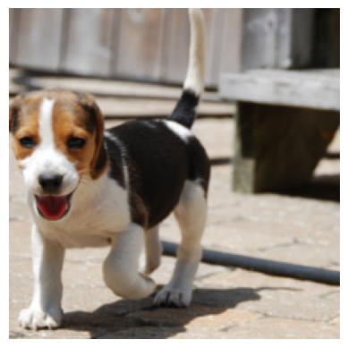
# Randomly select a data number
i = np.random.randint(len(train_dataset))

# convert train.data to a numpy array and store the 0th data in the minibatch named img
img = train_dataset[i][0].numpy().transpose(1,2,0) * IMG_STD + IMG_MEAN

# [0,1] clip: rewrite values less than or equal to 0 and greater than 1 to 0 and 1, respectively
img = np.clip(img, 0.0, 1.0)

# Corresponding correct answer value
label = train_dataset[i][1]

# Print label: label string (directory name) is stored in train_dataset.classes
print('label:', label, '\t', train_dataset.classes[label])

# Display with imshow
plt.imshow(img)
plt.axis('off') # no axis displayed
plt.show()
label: 4 beagle
Creating a DataLoader.
Creates an instance of torch.utils.data.DataLoader.
The arguments are
DataSet: different for train and val
minibatch size: set to 64 below. The size is often set to \(2^n\) for efficient parallel computation, but it does not have to be.
shuffle: Whether the order is randomly reordered or not
drop_last: whether to drop the last mini-batch or not, depends on train and val
num_workers: number of CPUs
pin_memory: whether to use past information in memory
[ ]:
import os

# Fix the seed
torch.manual_seed(0)

# Set yje size of mini-batches
batch_size = 64

# Define Data Loader
train_loader = torch.utils.data.DataLoader(train_dataset, batch_size, shuffle=True, drop_last=True, num_workers=os.cpu_count(), pin_memory=True)
val_loader = torch.utils.data.DataLoader(val_dataset, batch_size, shuffle=True, num_workers=os.cpu_count(), pin_memory=True)
DataLoader is an 「iterable」 type class, so it is intended to be used in a 「for」 statement.
[ ]:
for i, (x,y) in enumerate(val_loader):
    print(f'i:{i}\t x.shape: {x.shape}\t y.shape: {y.shape}')
i:0      x.shape: torch.Size([64, 3, 224, 224])  y.shape: torch.Size([64])
i:1      x.shape: torch.Size([64, 3, 224, 224])  y.shape: torch.Size([64])
i:2      x.shape: torch.Size([64, 3, 224, 224])  y.shape: torch.Size([64])
i:3      x.shape: torch.Size([64, 3, 224, 224])  y.shape: torch.Size([64])
i:4      x.shape: torch.Size([64, 3, 224, 224])  y.shape: torch.Size([64])
i:5      x.shape: torch.Size([64, 3, 224, 224])  y.shape: torch.Size([64])
i:6      x.shape: torch.Size([64, 3, 224, 224])  y.shape: torch.Size([64])
i:7      x.shape: torch.Size([64, 3, 224, 224])  y.shape: torch.Size([64])
i:8      x.shape: torch.Size([64, 3, 224, 224])  y.shape: torch.Size([64])
i:9      x.shape: torch.Size([64, 3, 224, 224])  y.shape: torch.Size([64])
i:10     x.shape: torch.Size([64, 3, 224, 224])  y.shape: torch.Size([64])
i:11     x.shape: torch.Size([64, 3, 224, 224])  y.shape: torch.Size([64])
i:12     x.shape: torch.Size([64, 3, 224, 224])  y.shape: torch.Size([64])
i:13     x.shape: torch.Size([64, 3, 224, 224])  y.shape: torch.Size([64])
i:14     x.shape: torch.Size([64, 3, 224, 224])  y.shape: torch.Size([64])
i:15     x.shape: torch.Size([64, 3, 224, 224])  y.shape: torch.Size([64])
i:16     x.shape: torch.Size([64, 3, 224, 224])  y.shape: torch.Size([64])
i:17     x.shape: torch.Size([64, 3, 224, 224])  y.shape: torch.Size([64])
i:18     x.shape: torch.Size([64, 3, 224, 224])  y.shape: torch.Size([64])
i:19     x.shape: torch.Size([64, 3, 224, 224])  y.shape: torch.Size([64])
i:20     x.shape: torch.Size([64, 3, 224, 224])  y.shape: torch.Size([64])
i:21     x.shape: torch.Size([64, 3, 224, 224])  y.shape: torch.Size([64])
i:22     x.shape: torch.Size([64, 3, 224, 224])  y.shape: torch.Size([64])
i:23     x.shape: torch.Size([6, 3, 224, 224])   y.shape: torch.Size([6])
It can also be used in combination with iter() and next().
[ ]:
iteration = iter(val_loader)

x, y = next(iteration)
print(f'y: {y}')

x, y = next(iteration)
print(f'y: {y}')
y: tensor([35,  6, 22,  7, 18,  3,  5, 21, 16, 16,  5, 33, 13,  2, 11, 11, 12,  5,
         9, 24, 18, 24,  5, 35, 18,  9,  2, 17, 29, 15,  7, 36, 16, 36,  2,  4,
        32, 32, 20, 19, 19, 11, 25, 22, 30,  6,  4,  8,  3, 28,  9, 12, 10, 26,
        28, 16, 24, 24, 32,  3, 20, 16,  5, 27])
y: tensor([16, 18,  8, 31,  9, 35, 25, 13,  7, 23, 19, 16, 16,  4,  0,  1,  0, 22,
        10,  9, 19, 27,  6,  7,  1,  3, 14,  0,  0,  1, 18, 22,  0, 34, 30,  7,
         0, 24, 35, 21,  1, 22,  2, 15,  8, 24, 12, 36,  0, 32, 22, 34, 14, 25,
        18, 21, 10,  9, 11,  9, 32, 33,  3, 11])
6.3. Model building and training
Next, we create a deep learning model called ResNet18 and train it.
Basically, the model is built using the torch.nn.module() class, but this time we will use a pre-defined model with only the output part modified. We can also use parameters that have already been trained on ImageNet, which contains millions of images.
While training a deep learning model from scratch often requires tens of thousands of images or more of data, a model with practical accuracy can be obtained with a small amount of data by using a pre-trained model as follows.
ResNet is characterized by a structure in which data is branched, skipped several layers, and then merged, as shown in the figure below ResNet18 is a ResNet with 17 convolution layers and one fully connected layer (Dense, Affine).
In this case, the last layer (the rightmost layer) labeled fc10 is replaced so that the output has 37 dimensions, the same as the number of target classes.
Figure source https://i.imgur.com/bpo9v4r.png
※A list of models and parameters provided by torchvision can be found here. Lighter and better performing models, such as EfficientNet, are also available.
[ ]:
import torch.nn as nn
from torchvision.models import resnet18

# Read resnet18 with the weight 'ResNet18_Weights.IMAGENET1K_V1' to see the structure
base_model = resnet18(weights='ResNet18_Weights.IMAGENET1K_V1')

base_model
Downloading: "https://download.pytorch.org/models/resnet18-f37072fd.pth" to /root/.cache/torch/hub/checkpoints/resnet18-f37072fd.pth
100%|██████████| 44.7M/44.7M [00:00<00:00, 102MB/s]
ResNet(
  (conv1): Conv2d(3, 64, kernel_size=(7, 7), stride=(2, 2), padding=(3, 3), bias=False)
  (bn1): BatchNorm2d(64, eps=1e-05, momentum=0.1, affine=True, track_running_stats=True)
  (relu): ReLU(inplace=True)
  (maxpool): MaxPool2d(kernel_size=3, stride=2, padding=1, dilation=1, ceil_mode=False)
  (layer1): Sequential(
    (0): BasicBlock(
      (conv1): Conv2d(64, 64, kernel_size=(3, 3), stride=(1, 1), padding=(1, 1), bias=False)
      (bn1): BatchNorm2d(64, eps=1e-05, momentum=0.1, affine=True, track_running_stats=True)
      (relu): ReLU(inplace=True)
      (conv2): Conv2d(64, 64, kernel_size=(3, 3), stride=(1, 1), padding=(1, 1), bias=False)
      (bn2): BatchNorm2d(64, eps=1e-05, momentum=0.1, affine=True, track_running_stats=True)
    )
    (1): BasicBlock(
      (conv1): Conv2d(64, 64, kernel_size=(3, 3), stride=(1, 1), padding=(1, 1), bias=False)
      (bn1): BatchNorm2d(64, eps=1e-05, momentum=0.1, affine=True, track_running_stats=True)
      (relu): ReLU(inplace=True)
      (conv2): Conv2d(64, 64, kernel_size=(3, 3), stride=(1, 1), padding=(1, 1), bias=False)
      (bn2): BatchNorm2d(64, eps=1e-05, momentum=0.1, affine=True, track_running_stats=True)
    )
  )
  (layer2): Sequential(
    (0): BasicBlock(
      (conv1): Conv2d(64, 128, kernel_size=(3, 3), stride=(2, 2), padding=(1, 1), bias=False)
      (bn1): BatchNorm2d(128, eps=1e-05, momentum=0.1, affine=True, track_running_stats=True)
      (relu): ReLU(inplace=True)
      (conv2): Conv2d(128, 128, kernel_size=(3, 3), stride=(1, 1), padding=(1, 1), bias=False)
      (bn2): BatchNorm2d(128, eps=1e-05, momentum=0.1, affine=True, track_running_stats=True)
      (downsample): Sequential(
        (0): Conv2d(64, 128, kernel_size=(1, 1), stride=(2, 2), bias=False)
        (1): BatchNorm2d(128, eps=1e-05, momentum=0.1, affine=True, track_running_stats=True)
      )
    )
    (1): BasicBlock(
      (conv1): Conv2d(128, 128, kernel_size=(3, 3), stride=(1, 1), padding=(1, 1), bias=False)
      (bn1): BatchNorm2d(128, eps=1e-05, momentum=0.1, affine=True, track_running_stats=True)
      (relu): ReLU(inplace=True)
      (conv2): Conv2d(128, 128, kernel_size=(3, 3), stride=(1, 1), padding=(1, 1), bias=False)
      (bn2): BatchNorm2d(128, eps=1e-05, momentum=0.1, affine=True, track_running_stats=True)
    )
  )
  (layer3): Sequential(
    (0): BasicBlock(
      (conv1): Conv2d(128, 256, kernel_size=(3, 3), stride=(2, 2), padding=(1, 1), bias=False)
      (bn1): BatchNorm2d(256, eps=1e-05, momentum=0.1, affine=True, track_running_stats=True)
      (relu): ReLU(inplace=True)
      (conv2): Conv2d(256, 256, kernel_size=(3, 3), stride=(1, 1), padding=(1, 1), bias=False)
      (bn2): BatchNorm2d(256, eps=1e-05, momentum=0.1, affine=True, track_running_stats=True)
      (downsample): Sequential(
        (0): Conv2d(128, 256, kernel_size=(1, 1), stride=(2, 2), bias=False)
        (1): BatchNorm2d(256, eps=1e-05, momentum=0.1, affine=True, track_running_stats=True)
      )
    )
    (1): BasicBlock(
      (conv1): Conv2d(256, 256, kernel_size=(3, 3), stride=(1, 1), padding=(1, 1), bias=False)
      (bn1): BatchNorm2d(256, eps=1e-05, momentum=0.1, affine=True, track_running_stats=True)
      (relu): ReLU(inplace=True)
      (conv2): Conv2d(256, 256, kernel_size=(3, 3), stride=(1, 1), padding=(1, 1), bias=False)
      (bn2): BatchNorm2d(256, eps=1e-05, momentum=0.1, affine=True, track_running_stats=True)
    )
  )
  (layer4): Sequential(
    (0): BasicBlock(
      (conv1): Conv2d(256, 512, kernel_size=(3, 3), stride=(2, 2), padding=(1, 1), bias=False)
      (bn1): BatchNorm2d(512, eps=1e-05, momentum=0.1, affine=True, track_running_stats=True)
      (relu): ReLU(inplace=True)
      (conv2): Conv2d(512, 512, kernel_size=(3, 3), stride=(1, 1), padding=(1, 1), bias=False)
      (bn2): BatchNorm2d(512, eps=1e-05, momentum=0.1, affine=True, track_running_stats=True)
      (downsample): Sequential(
        (0): Conv2d(256, 512, kernel_size=(1, 1), stride=(2, 2), bias=False)
        (1): BatchNorm2d(512, eps=1e-05, momentum=0.1, affine=True, track_running_stats=True)
      )
    )
    (1): BasicBlock(
      (conv1): Conv2d(512, 512, kernel_size=(3, 3), stride=(1, 1), padding=(1, 1), bias=False)
      (bn1): BatchNorm2d(512, eps=1e-05, momentum=0.1, affine=True, track_running_stats=True)
      (relu): ReLU(inplace=True)
      (conv2): Conv2d(512, 512, kernel_size=(3, 3), stride=(1, 1), padding=(1, 1), bias=False)
      (bn2): BatchNorm2d(512, eps=1e-05, momentum=0.1, affine=True, track_running_stats=True)
    )
  )
  (avgpool): AdaptiveAvgPool2d(output_size=(1, 1))
  (fc): Linear(in_features=512, out_features=1000, bias=True)
)
The nn.modele class is used to create a model with a modified output section.
We can create a new model class (e.g. Resnet) by inheriting from nn.modele class as
class Resnet(nn.Module):.
    def __init__(self):.
        # Initialize the inherited nn.Module (invoke __init__() in nn.Module)
        super(Resnet, self). __init__()
        # Define model parameters, etc.
        .......
    def __call__(self, x):.
        # Define output y
        ........
        return y
The output layers can be modified by
base_model.fc = nn.Linear(in_features=512, out_features=37, bias=True)
[ ]:
import torch.nn as nn

class Resnet(nn.Module):
    def __init__(self):
        # Initialize nn.Module
        super(Resnet, self).__init__()

        base_model = resnet18(weights='ResNet18_Weights.IMAGENET1K_V1')
        base_model.fc = nn.Linear(in_features=512, out_features=37, bias=True)
        self.model = base_model

    def __call__(self, x):
        y = self.model(x)
        return y
[ ]:
import torch.optim as optim

# set device 'cpu' or 'cuda' (GPU)
device = torch.device("cuda")

# Generate model and send to device
model = Resnet().to(device)

# Set optimization method
optimizer = torch.optim.Adam(model.parameters(), lr=0.002)
Learning function.
The learning process (loss function, accuracy with respect to evaluation data, etc.) is complicated, but the learning itself is as described in this notebook.
[ ]:
import datetime # Time-related library
import torch.nn.functional as F


def train(model, epoch_num=5):
    # Start learning
    st = datetime.datetime.now() # start time
    print('training started')

    # Execute the following for epoch_num times
    for epoch in range(epoch_num):

        # Variables for recording learning
        total_loss = 0.0
        train_total = 0

        # Set the model to learning mode
        model.train()

        # 1 epoch learning with train_loader
        for i, (x,t) in enumerate(train_loader):

            # Send input data x and correct value t to device: a little faster if non_blocking=True
            x, t = x.to(device, non_blocking=True), t.to(device, non_blocking=True)

            # Initialize gradient calculation
            optimizer.zero_grad()

            # Calculate output values
            y = model(x)

            # Compute loss function: 37 dimensions, t: integer value from which F.cross_entropy(y, t) computes cross-entropy
            loss = F.cross_entropy(y, t)

            # Perform gradient calculation and optimization
            loss.backward()
            optimizer.step()

            # For recording learning
            total_loss += loss.item() * len(t)
            train_total += len(t)

        # Recording the learning.
        mean_loss = total_loss/train_total
        if (epoch+1) % 1 == 0: # Since %1 is the remainder divided by 1, we compute every epoch after all.
            ed = datetime.datetime.now()
            correct = 0
            val_total = 0
            model.eval() # Evaluataion mode
            for i, (x,t) in enumerate (val_loader):
                x, t = x.to(device, non_blocking=True), t.to(device, non_blocking=True)
                y = model(x)
                correct += (y.argmax(axis=1) == t).float().sum()
                val_total += len(t)

            accuracy = correct / val_total

            print(f'epoch:{epoch+1}\t mean loss:: {mean_loss}\t time:{ed-st}\t val_accuracy:{accuracy}')
            st = datetime.datetime.now()
Transfer learning
Here we use a slightly difficult technique called transfer learning. This means that newly added parameters are learned with requires_grad = True and and the learned parameters are learned with requires_grad = False. This prevents the learned parameters from being corrupted.
In our case, only the modified output layer is trained.
The naming of layers varies by model, so it is necessary to look carefully at the structure of the model.
[ ]:
# Fixed parameters: Only the output layer can be trained.
for name, param in model.named_parameters():
    if '.fc' in name:
        param.requires_grad = True
        print(f'{name}: {True}')
    else:
        param.requires_grad = False
        # print(f'{name}: {False}')

# # This time it works fine, but it may not work well under different photographic conditions.
# # Fixed parameters: only batch normalization layer and output layer can be trained
# for name, param in model.named_parameters():
#     if ('.bn' in name) or ('.fc' in name):
#         param.requires_grad = True
#         print(f'{name}: {True}')
#     else:
#         param.requires_grad = False
#         print(f'{name}: {False}')
model.fc.weight: True
model.fc.bias: True
[ ]:
train(model, epoch_num=2)
training started
epoch:1  mean loss:: 1.3117052656800852  time:0:00:43.357089     val_accuracy:0.877537190914154
epoch:2  mean loss:: 0.47171791578116623         time:0:00:42.241236     val_accuracy:0.9025710225105286
Fine Tuning.
Continue to train all layers.
[ ]:
# Unfixing parameters
for name, param in model.named_parameters():
    param.requires_grad = True
Note that the learning coefficient is very small, 0.0001. This is also to ensure that the learned parameters are not corrupted.
[ ]:
optimizer = torch.optim.Adam(model.parameters(), lr=0.0001)
train(model, epoch_num=3)
training started
epoch:1  mean loss:: 0.3151126855417438  time:0:00:48.903363     val_accuracy:0.9208389520645142
epoch:2  mean loss:: 0.16125210269313792         time:0:00:49.795584     val_accuracy:0.9215155243873596
epoch:3  mean loss:: 0.11092852760592233         time:0:00:48.787167     val_accuracy:0.9255750775337219
6.4. Prediction on test data
[ ]:
model.to('cpu')
model.eval()
for i, (x,t) in enumerate (val_loader):
y = model(x)
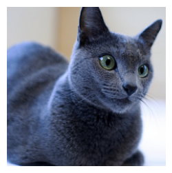
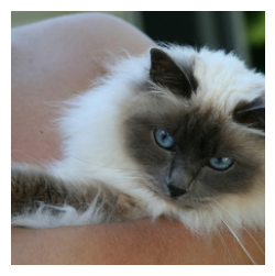
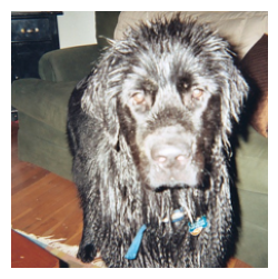
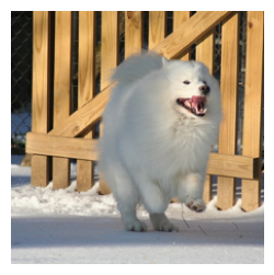
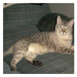
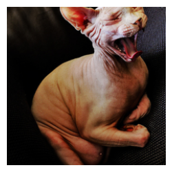
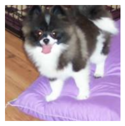
for i in range(10):
print('predicted label:', val_dataset.classes[y.argmax(axis=1).numpy()[i]],
'\t correct label:', val_dataset.classes[t.numpy()[i]])
# convert train.data to a numpy array and store the 0th data in a variable named img
img = x[i].numpy().transpose(1,2,0) * IMG_STD + IMG_MEAN
img = np.clip(img, 0.0, 1.0)
# Show the image by imshow
plt.figure(figsize=(3,3))
plt.imshow(img)
plt.axis('off')
plt.show()
break
predicted label: russian_blue correct label: russian_blue
predicted label: birman correct label: birman
predicted label: newfoundland correct label: newfoundland
predicted label: great_pyrenees correct label: samoyed
predicted label: egyptian_mau correct label: bengal
predicted label: sphynx correct label: sphynx
predicted label: ragdoll correct label: pomeranian
predicted label: shiba_inu correct label: shiba_inu
predicted label: american_pit_bull_terrier correct label: american_pit_bull_terrier
predicted label: saint_bernard correct label: saint_bernard
[ ]: