5. Introduction to deep learning
Notebook (Exercise) for this section (open in another tab)
Video (21 min)
5.1. Flow of regression analysis by deep learning
Let’s follow the flow of deep learning, using the simplest machine learning problem, regression analysis (prediction of numerical values) as an example.
The flow of machine learning is as follows, that is not limited to regression problems.
A “model” in machine learning is a “function” that makes some predictions on input data. A function has parameters, and once the parameters are determined, predictions can be made. If appropriate parameters are obtained by learning with data, appropriate predictions can be expected for new data.
Data acquisition and preprocessing
In preprocessing, input and correct answer data are prepared for supervised learning. The data is then formatted according to the model to be used, and the data scattering is standardized. We also separate the data into training data and evaluation data so that we can evaluate the performance of the model. Alternatively, the data may be divided into three groups: training data, evaluation data, and test data for generalization evaluation.
Create a neural network model
The model of regression analysis is a function \(\hat{y} = f(x, \theta)\) that predicts an approximation \(\hat{y}\) of \(y\) for an input \(x\). Note that \(\theta\) is a parameter that is updated by training. In addition to the parameters to be trained, neural networks have various parameters related to the structure of the model, such as the number of layers, the size of each layer, the activation function, and the dropout ratio. Since these structural parameters are not improved in training process, they are called hyperparameters to distinguish them from the parameters to be trained. In other words, a neural network has many hyperparameters that should be predetermined.
Training and evaluation of neural network models
Machine learning, also called statistical machine learning, uses data to optimize model parameters so that predictions can be made for new data. The same is true for deep learning, and optimization is performed using training data so that the error between the model’s prediction and the correct value becomes small. However, simply optimizing a model with high expressive power, such as deep learning models, may result in over-optimization for the training data, resulting in a decline in predictive performance (generalization performance) for new data. This situation is called “overfitting”. To avoid overfitting, various ideas have been proposed for neural network structures and for learning methods.
The evaluation data is used to evaluate the generalization performance as well as to adjust the non-learned parameters of the model (called hyper-parameters). The test data are used purely for the evaluation of generalization performance.
Applying Neural Network Models to New Data
The model \(f(x,\theta)\) obtained from training is used to predict values for test data and new input data \(x\).
Deep learnibng frameworks
Deep learning frameworks offer building blocks for designing, training, and validating deep neural networks through a high-level programming interface. The most popular libraries for deep learning are TensorFlow and PyTorch. TensorFlow is suitable for practical use, especially when used with a partial library called Keras, because it is easy to describe and has a function to be loaded on terminal devices. PyTorch is highly customizable and is often used in research. This notebook uses TensorFlow-Keras, which is the easiest to implement, to train a neural network model for regression problems.
[ ]:
# import libraries
import numpy as np # numpy is a library for numerical analysis.
import pandas as pd # pandas is library for data analysis
import matplotlib.pyplot as plt # a library for plotting graphs
5.2. Data acquisition and preprocessing
Load a dataset about average house prices in Boston from this csv file.
[ ]:
# Dataset download: A file named BostonHousing.csv is downloaded to the home directory (/content/)
!wget 'https://raw.githubusercontent.com/selva86/datasets/master/BostonHousing.csv'

# Read dataset: Read csv file and store contents in variable df of Pandas DataFrame class.
# header=0: Specifies that row 0 is a column name.
# sep=',': Specifies that the delimiter is a comma.
df = pd.read_csv('/content/BostonHousing.csv', header=0, sep=',')

# Display df
df
--2024-03-14 01:53:51--  https://raw.githubusercontent.com/selva86/datasets/master/BostonHousing.csv
Resolving raw.githubusercontent.com (raw.githubusercontent.com)... 185.199.108.133, 185.199.109.133, 185.199.110.133, ...
Connecting to raw.githubusercontent.com (raw.githubusercontent.com)|185.199.108.133|:443... connected.
HTTP request sent, awaiting response... 200 OK
Length: 35735 (35K) [text/plain]
Saving to: ‘BostonHousing.csv’

BostonHousing.csv   100%[===================>]  34.90K  --.-KB/s    in 0.003s

2024-03-14 01:53:52 (10.1 MB/s) - ‘BostonHousing.csv’ saved [35735/35735]
| crim | zn | indus | chas | nox | rm | age | dis | rad | tax | ptratio | b | lstat | medv | |
|---|---|---|---|---|---|---|---|---|---|---|---|---|---|---|
| 0 | 0.00632 | 18.0 | 2.31 | 0 | 0.538 | 6.575 | 65.2 | 4.0900 | 1 | 296 | 15.3 | 396.90 | 4.98 | 24.0 |
| 1 | 0.02731 | 0.0 | 7.07 | 0 | 0.469 | 6.421 | 78.9 | 4.9671 | 2 | 242 | 17.8 | 396.90 | 9.14 | 21.6 |
| 2 | 0.02729 | 0.0 | 7.07 | 0 | 0.469 | 7.185 | 61.1 | 4.9671 | 2 | 242 | 17.8 | 392.83 | 4.03 | 34.7 |
| 3 | 0.03237 | 0.0 | 2.18 | 0 | 0.458 | 6.998 | 45.8 | 6.0622 | 3 | 222 | 18.7 | 394.63 | 2.94 | 33.4 |
| 4 | 0.06905 | 0.0 | 2.18 | 0 | 0.458 | 7.147 | 54.2 | 6.0622 | 3 | 222 | 18.7 | 396.90 | 5.33 | 36.2 |
| ... | ... | ... | ... | ... | ... | ... | ... | ... | ... | ... | ... | ... | ... | ... |
| 501 | 0.06263 | 0.0 | 11.93 | 0 | 0.573 | 6.593 | 69.1 | 2.4786 | 1 | 273 | 21.0 | 391.99 | 9.67 | 22.4 |
| 502 | 0.04527 | 0.0 | 11.93 | 0 | 0.573 | 6.120 | 76.7 | 2.2875 | 1 | 273 | 21.0 | 396.90 | 9.08 | 20.6 |
| 503 | 0.06076 | 0.0 | 11.93 | 0 | 0.573 | 6.976 | 91.0 | 2.1675 | 1 | 273 | 21.0 | 396.90 | 5.64 | 23.9 |
| 504 | 0.10959 | 0.0 | 11.93 | 0 | 0.573 | 6.794 | 89.3 | 2.3889 | 1 | 273 | 21.0 | 393.45 | 6.48 | 22.0 |
| 505 | 0.04741 | 0.0 | 11.93 | 0 | 0.573 | 6.030 | 80.8 | 2.5050 | 1 | 273 | 21.0 | 396.90 | 7.88 | 11.9 |
506 rows × 14 columns
The data consists of 506 rows and 14 columns.
Of these, medv (average home price in each district) is used as the objective value (correct answer), and the remaining 13 items, excluding the categorical variables chas and rad and the ethically problematic b (percentage of blacks), are used as explanatory variables.
This creates data for a regression problem that predicts a one-dimensional value, the average home price in the district, from 10 dimensions of input data for each district.
[ ]:
# Let x be df excluding the columns chas, rad, b, and medv. axis=1 specifies "column".
x = df.drop(['chas', 'rad', 'b', 'medv'], axis=1)

# Let y be the column of medv out of df
y = df['medv']

# Display the first 5 rows of x
x.head()
| crim | zn | indus | nox | rm | age | dis | tax | ptratio | lstat | |
|---|---|---|---|---|---|---|---|---|---|---|
| 0 | 0.00632 | 18.0 | 2.31 | 0.538 | 6.575 | 65.2 | 4.0900 | 296 | 15.3 | 4.98 |
| 1 | 0.02731 | 0.0 | 7.07 | 0.469 | 6.421 | 78.9 | 4.9671 | 242 | 17.8 | 9.14 |
| 2 | 0.02729 | 0.0 | 7.07 | 0.469 | 7.185 | 61.1 | 4.9671 | 242 | 17.8 | 4.03 |
| 3 | 0.03237 | 0.0 | 2.18 | 0.458 | 6.998 | 45.8 | 6.0622 | 222 | 18.7 | 2.94 |
| 4 | 0.06905 | 0.0 | 2.18 | 0.458 | 7.147 | 54.2 | 6.0622 | 222 | 18.7 | 5.33 |
The input data are linearly transformed so that the mean is 0 and the variance is 1 for each item.
[ ]:
mean = x.mean(axis=0)    # column-wise mean
standard = x.std(axis=0) # standard deviation per column
x = (x-mean)/standard    # standardized to mean 0, variance 1
Of the data, 80% is randomly selected as training data, and the remaining 20% is used as test data to evaluate the training results.
[ ]:
# Load sklearn's train_test_split function
from sklearn.model_selection import train_test_split

# Fix the random seed to 0 to get the same result every time
np.random.seed(0)

# Split data into input data for training, input data for test data, correct answer for training data, and correct answer for test data with train_test_split function
x_train, x_test, y_train, y_test = train_test_split(x, y, test_size=0.2)

# Display the first 5 rows of input data for training
x_train.head()
| crim | zn | indus | nox | rm | age | dis | tax | ptratio | lstat | |
|---|---|---|---|---|---|---|---|---|---|---|
| 220 | -0.378471 | -0.487240 | -0.719610 | -0.411598 | 0.948405 | 0.707847 | -0.443244 | -0.600682 | -0.487557 | -0.412132 |
| 71 | -0.401645 | -0.487240 | -0.047633 | -1.222799 | -0.460613 | -1.814457 | 0.708672 | -0.612548 | 0.343873 | -0.388326 |
| 240 | -0.406931 | 0.799074 | -0.904732 | -1.093352 | 0.871549 | -0.507122 | 1.206746 | -0.642216 | -0.857081 | -0.178274 |
| 6 | -0.409837 | 0.048724 | -0.476182 | -0.264892 | -0.388027 | -0.070159 | 0.838414 | -0.576948 | -1.503749 | -0.031237 |
| 417 | 2.595705 | -0.487240 | 1.014995 | 1.072726 | -1.395688 | 0.729163 | -1.019866 | 1.529413 | 0.805778 | 1.958664 |
[ ]:
# Display the type as an array of input data and correct answer data for training: 404 rows of data
x_train.shape, y_train.shape
((404, 10), (404,))
5.3. Training Neural Networks with TensorFlow-Keras
Creating a model
Using a class called Sequential, we created the following model
10 input dimensions — 1000 dimensions — 800 dimensions — 100 dimensions — 1 output dimension
model.add(Dense(1000, activation = 'relu'))
adds a layer with 1000 neurons and ReLU activation function.
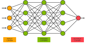
A neural network transmits data from the input (leftmost) to a layer of neurons arranged vertically in a row and transforms them in sequence, as shown in the figure below.
A single neuron (a vertex in the graph) performs a 「linear sum + constant」 on the output \((x_1, x_2, \cdots, x_n)\) of the vertices on the left.
\[a = w_1x_1 +w_2 x_2 + \cdots+ w_n x_n + b\]and outputs the value \(y =f(a)\) after applying the activation function \(f\) to it.
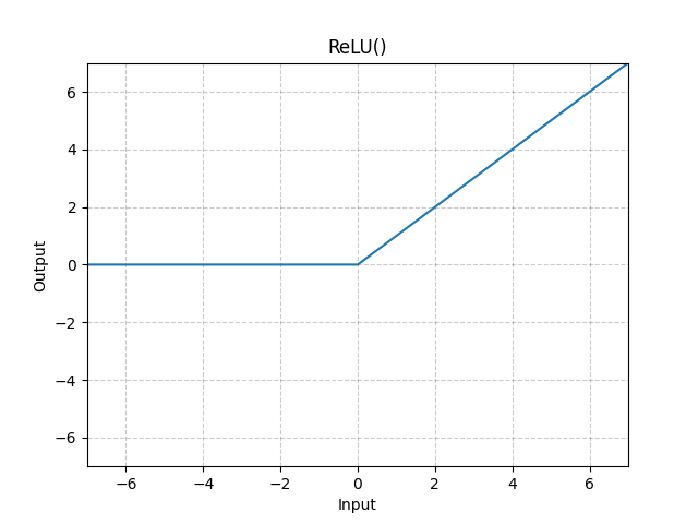
The activation function is a nonlinear function, typically ReLU (Rectified Linear Unit \(= \max(x,0)\)) is used.
Neural Networks: Figure Source https://vitalflux.com/wp-content/uploads/2023/02/Sklearn-Neural-Network-MLPRegressor-Regression-Model–300x166.png
ReLU: Figure Source https://pytorch.org/docs/stable/_images/ReLU.png
[ ]:
'''
Generating a Neural Network Model
The model consists of
Input (10 dimensions) - 1000 dimensions - 800 dimensions - 100 dimensions - Predictions (1 dimension)
Sequential() is a class of models that can be written without branching from the input
Dense() is the all-connecting (affine) layer
activation is the activation function, ReLU is used here
'''

from tensorflow.keras.models import Sequential
from tensorflow.keras.layers import Dense

# Create an instance of the Sequential class and name it as“model”
model = Sequential()

# Add a 1000 dimensional layer to model; activation function is ReLU
model.add(Dense(1000, activation = 'relu'))

# Add a 800 dimensional layer to model; activation function is ReLU
model.add(Dense(800, activation = 'relu'))

# Add a 100 dimensional layer to model; activation function is ReLU
model.add(Dense(100, activation = 'relu'))

# Add a 1-dimensional layer to model; no activation function is applied to the last layer for the regression problem
model.add(Dense(1))
Compile
Prepare for training by executing the compile method of the Sequential class. The optimization method is Adam, an improved version of SGD (Stochastic Gradient Descent), and the error function is the mean squared error.
[ ]:
'''
Compile the model
Compiling the model prepares inverse propagation.
Specify Adam as the optimization function
Mean squared error is specified as the error function
'''

from tensorflow.keras.optimizers import Adam

# Compiling with optimization function Adam, learning coefficient 1e-3 = 0.001, and mean squared error (average of the squares of the errors) as the loss function
model.compile(Adam(learning_rate=1e-3), loss="mean_squared_error")
Learning
Learning is performed using a method of the Sequential class called fit.
The training data is used for 150 epochs (i.e., 150 rounds of the dataset), and then evaluated on test data. The batch size of 128 means that 128 data are input at a time and the parameters are updated.
In this case, there are 404 data in the training data set, so \(404/128=4\) (rounded up) updates are performed per epoch. There are 150 epochs, so the total number of updates is \(4\times 150=600\) times.
[ ]:
'''
train on training data with function "fit" and evaluate on test data

batch_size: Number of data in a mini-batch
epochs: Number of times to process all the data. 1 epoch = 1 round
verbose: Display format, 0 means nothing is displayed, 1 means training results are displayed at each epoch
validation _data: data for evaluation (here we use the test data as is, since we do not adjust the hyperparameters)
'''
history = model.fit(x_train, y_train, batch_size=128, epochs=150, verbose=1,
          validation_data=(x_test, y_test))
Epoch 1/150
4/4 [==============================] - 1s 98ms/step - loss: 542.2038 - val_loss: 378.2771
Epoch 2/150
4/4 [==============================] - 0s 35ms/step - loss: 313.3249 - val_loss: 142.4200
Epoch 3/150
4/4 [==============================] - 0s 33ms/step - loss: 120.3861 - val_loss: 167.2755
Epoch 4/150
4/4 [==============================] - 0s 38ms/step - loss: 112.8099 - val_loss: 76.4208
Epoch 5/150
4/4 [==============================] - 0s 34ms/step - loss: 42.2795 - val_loss: 71.8820
Epoch 6/150
4/4 [==============================] - 0s 40ms/step - loss: 45.0763 - val_loss: 58.8306
Epoch 7/150
4/4 [==============================] - 0s 36ms/step - loss: 29.7077 - val_loss: 47.6159
Epoch 8/150
4/4 [==============================] - 0s 78ms/step - loss: 26.8966 - val_loss: 44.8242
Epoch 9/150
4/4 [==============================] - 0s 43ms/step - loss: 24.5714 - val_loss: 36.3940
Epoch 10/150
4/4 [==============================] - 0s 36ms/step - loss: 19.3088 - val_loss: 34.3080
Epoch 11/150
4/4 [==============================] - 0s 38ms/step - loss: 17.4799 - val_loss: 31.7423
Epoch 12/150
4/4 [==============================] - 0s 40ms/step - loss: 16.1699 - val_loss: 32.1581
Epoch 13/150
4/4 [==============================] - 0s 79ms/step - loss: 15.8482 - val_loss: 31.9483
Epoch 14/150
4/4 [==============================] - 0s 39ms/step - loss: 15.0977 - val_loss: 30.9777
Epoch 15/150
4/4 [==============================] - 0s 34ms/step - loss: 14.6053 - val_loss: 30.4021
Epoch 16/150
4/4 [==============================] - 0s 38ms/step - loss: 13.8320 - val_loss: 30.5984
Epoch 17/150
4/4 [==============================] - 0s 36ms/step - loss: 13.3431 - val_loss: 30.5575
Epoch 18/150
4/4 [==============================] - 0s 39ms/step - loss: 12.9117 - val_loss: 29.3249
Epoch 19/150
4/4 [==============================] - 0s 34ms/step - loss: 12.6846 - val_loss: 28.2872
Epoch 20/150
4/4 [==============================] - 0s 35ms/step - loss: 12.1732 - val_loss: 27.7082
Epoch 21/150
4/4 [==============================] - 0s 36ms/step - loss: 11.9274 - val_loss: 27.1071
Epoch 22/150
4/4 [==============================] - 0s 36ms/step - loss: 11.6732 - val_loss: 26.6342
Epoch 23/150
4/4 [==============================] - 0s 35ms/step - loss: 11.4140 - val_loss: 25.2945
Epoch 24/150
4/4 [==============================] - 0s 39ms/step - loss: 11.2454 - val_loss: 25.4208
Epoch 25/150
4/4 [==============================] - 0s 40ms/step - loss: 10.9239 - val_loss: 25.6217
Epoch 26/150
4/4 [==============================] - 0s 37ms/step - loss: 10.7363 - val_loss: 25.1891
Epoch 27/150
4/4 [==============================] - 0s 36ms/step - loss: 10.5209 - val_loss: 25.5208
Epoch 28/150
4/4 [==============================] - 0s 40ms/step - loss: 10.1774 - val_loss: 24.6743
Epoch 29/150
4/4 [==============================] - 0s 40ms/step - loss: 10.0736 - val_loss: 24.5310
Epoch 30/150
4/4 [==============================] - 0s 36ms/step - loss: 10.0467 - val_loss: 24.2703
Epoch 31/150
4/4 [==============================] - 0s 37ms/step - loss: 9.9615 - val_loss: 23.8944
Epoch 32/150
4/4 [==============================] - 0s 41ms/step - loss: 9.5542 - val_loss: 24.5444
Epoch 33/150
4/4 [==============================] - 0s 36ms/step - loss: 9.5783 - val_loss: 25.8316
Epoch 34/150
4/4 [==============================] - 0s 37ms/step - loss: 9.7056 - val_loss: 24.9243
Epoch 35/150
4/4 [==============================] - 0s 35ms/step - loss: 9.3160 - val_loss: 22.9954
Epoch 36/150
4/4 [==============================] - 0s 37ms/step - loss: 9.2122 - val_loss: 22.8383
Epoch 37/150
4/4 [==============================] - 0s 38ms/step - loss: 8.7401 - val_loss: 23.8713
Epoch 38/150
4/4 [==============================] - 0s 37ms/step - loss: 8.5705 - val_loss: 22.4284
Epoch 39/150
4/4 [==============================] - 0s 52ms/step - loss: 8.3343 - val_loss: 21.0313
Epoch 40/150
4/4 [==============================] - 0s 54ms/step - loss: 8.7656 - val_loss: 21.2243
Epoch 41/150
4/4 [==============================] - 0s 51ms/step - loss: 8.5711 - val_loss: 23.2545
Epoch 42/150
4/4 [==============================] - 0s 54ms/step - loss: 8.3963 - val_loss: 23.4132
Epoch 43/150
4/4 [==============================] - 0s 62ms/step - loss: 8.2590 - val_loss: 20.8971
Epoch 44/150
4/4 [==============================] - 0s 59ms/step - loss: 8.1156 - val_loss: 21.2252
Epoch 45/150
4/4 [==============================] - 0s 51ms/step - loss: 7.7277 - val_loss: 22.2657
Epoch 46/150
4/4 [==============================] - 0s 51ms/step - loss: 7.4283 - val_loss: 21.8822
Epoch 47/150
4/4 [==============================] - 0s 57ms/step - loss: 7.1957 - val_loss: 20.5706
Epoch 48/150
4/4 [==============================] - 0s 51ms/step - loss: 7.2384 - val_loss: 20.1177
Epoch 49/150
4/4 [==============================] - 0s 60ms/step - loss: 7.0801 - val_loss: 20.8228
Epoch 50/150
4/4 [==============================] - 0s 52ms/step - loss: 6.8289 - val_loss: 20.3527
Epoch 51/150
4/4 [==============================] - 0s 56ms/step - loss: 7.1758 - val_loss: 19.0590
Epoch 52/150
4/4 [==============================] - 0s 45ms/step - loss: 7.0969 - val_loss: 20.2688
Epoch 53/150
4/4 [==============================] - 0s 35ms/step - loss: 6.7781 - val_loss: 21.1951
Epoch 54/150
4/4 [==============================] - 0s 36ms/step - loss: 6.7375 - val_loss: 19.5856
Epoch 55/150
4/4 [==============================] - 0s 37ms/step - loss: 6.9143 - val_loss: 19.4323
Epoch 56/150
4/4 [==============================] - 0s 32ms/step - loss: 6.3245 - val_loss: 21.3883
Epoch 57/150
4/4 [==============================] - 0s 36ms/step - loss: 6.4558 - val_loss: 20.5827
Epoch 58/150
4/4 [==============================] - 0s 36ms/step - loss: 6.2914 - val_loss: 19.7638
Epoch 59/150
4/4 [==============================] - 0s 41ms/step - loss: 6.0283 - val_loss: 19.5449
Epoch 60/150
4/4 [==============================] - 0s 34ms/step - loss: 6.0108 - val_loss: 19.6069
Epoch 61/150
4/4 [==============================] - 0s 36ms/step - loss: 5.6011 - val_loss: 19.2124
Epoch 62/150
4/4 [==============================] - 0s 39ms/step - loss: 5.5410 - val_loss: 19.0138
Epoch 63/150
4/4 [==============================] - 0s 33ms/step - loss: 5.6207 - val_loss: 19.3390
Epoch 64/150
4/4 [==============================] - 0s 41ms/step - loss: 5.5212 - val_loss: 19.2685
Epoch 65/150
4/4 [==============================] - 0s 38ms/step - loss: 5.2504 - val_loss: 19.3252
Epoch 66/150
4/4 [==============================] - 0s 35ms/step - loss: 5.5253 - val_loss: 19.4586
Epoch 67/150
4/4 [==============================] - 0s 35ms/step - loss: 5.3667 - val_loss: 20.0553
Epoch 68/150
4/4 [==============================] - 0s 36ms/step - loss: 5.3671 - val_loss: 18.5738
Epoch 69/150
4/4 [==============================] - 0s 46ms/step - loss: 5.1529 - val_loss: 19.0400
Epoch 70/150
4/4 [==============================] - 0s 38ms/step - loss: 4.9816 - val_loss: 19.5474
Epoch 71/150
4/4 [==============================] - 0s 36ms/step - loss: 4.9404 - val_loss: 18.4542
Epoch 72/150
4/4 [==============================] - 0s 37ms/step - loss: 4.8934 - val_loss: 18.6778
Epoch 73/150
4/4 [==============================] - 0s 36ms/step - loss: 4.7336 - val_loss: 19.7403
Epoch 74/150
4/4 [==============================] - 0s 37ms/step - loss: 4.7942 - val_loss: 18.5726
Epoch 75/150
4/4 [==============================] - 0s 42ms/step - loss: 4.6575 - val_loss: 18.3666
Epoch 76/150
4/4 [==============================] - 0s 40ms/step - loss: 4.6568 - val_loss: 18.2663
Epoch 77/150
4/4 [==============================] - 0s 37ms/step - loss: 4.7075 - val_loss: 17.9285
Epoch 78/150
4/4 [==============================] - 0s 34ms/step - loss: 4.5847 - val_loss: 19.0227
Epoch 79/150
4/4 [==============================] - 0s 36ms/step - loss: 4.6171 - val_loss: 18.5115
Epoch 80/150
4/4 [==============================] - 0s 35ms/step - loss: 4.5494 - val_loss: 18.1896
Epoch 81/150
4/4 [==============================] - 0s 40ms/step - loss: 4.3259 - val_loss: 18.4847
Epoch 82/150
4/4 [==============================] - 0s 35ms/step - loss: 4.2287 - val_loss: 17.6227
Epoch 83/150
4/4 [==============================] - 0s 37ms/step - loss: 4.2339 - val_loss: 17.5507
Epoch 84/150
4/4 [==============================] - 0s 35ms/step - loss: 4.1158 - val_loss: 18.1849
Epoch 85/150
4/4 [==============================] - 0s 34ms/step - loss: 4.2792 - val_loss: 18.7086
Epoch 86/150
4/4 [==============================] - 0s 35ms/step - loss: 4.1098 - val_loss: 17.2935
Epoch 87/150
4/4 [==============================] - 0s 36ms/step - loss: 4.7991 - val_loss: 17.8858
Epoch 88/150
4/4 [==============================] - 0s 38ms/step - loss: 5.1245 - val_loss: 17.1625
Epoch 89/150
4/4 [==============================] - 0s 34ms/step - loss: 4.4317 - val_loss: 16.4478
Epoch 90/150
4/4 [==============================] - 0s 41ms/step - loss: 4.4366 - val_loss: 18.0499
Epoch 91/150
4/4 [==============================] - 0s 39ms/step - loss: 4.4117 - val_loss: 16.6964
Epoch 92/150
4/4 [==============================] - 0s 38ms/step - loss: 4.2698 - val_loss: 17.3918
Epoch 93/150
4/4 [==============================] - 0s 36ms/step - loss: 3.9362 - val_loss: 18.7956
Epoch 94/150
4/4 [==============================] - 0s 37ms/step - loss: 3.9248 - val_loss: 16.6190
Epoch 95/150
4/4 [==============================] - 0s 41ms/step - loss: 4.0259 - val_loss: 16.4504
Epoch 96/150
4/4 [==============================] - 0s 35ms/step - loss: 3.6345 - val_loss: 17.3056
Epoch 97/150
4/4 [==============================] - 0s 43ms/step - loss: 3.8261 - val_loss: 17.0214
Epoch 98/150
4/4 [==============================] - 0s 39ms/step - loss: 3.8824 - val_loss: 17.5772
Epoch 99/150
4/4 [==============================] - 0s 35ms/step - loss: 3.5354 - val_loss: 17.1024
Epoch 100/150
4/4 [==============================] - 0s 37ms/step - loss: 3.6960 - val_loss: 16.8976
Epoch 101/150
4/4 [==============================] - 0s 33ms/step - loss: 3.7528 - val_loss: 16.9268
Epoch 102/150
4/4 [==============================] - 0s 38ms/step - loss: 3.8965 - val_loss: 17.5388
Epoch 103/150
4/4 [==============================] - 0s 33ms/step - loss: 3.7162 - val_loss: 16.4088
Epoch 104/150
4/4 [==============================] - 0s 42ms/step - loss: 3.6625 - val_loss: 17.6933
Epoch 105/150
4/4 [==============================] - 0s 35ms/step - loss: 3.7193 - val_loss: 18.8482
Epoch 106/150
4/4 [==============================] - 0s 35ms/step - loss: 3.4145 - val_loss: 17.5481
Epoch 107/150
4/4 [==============================] - 0s 40ms/step - loss: 3.8765 - val_loss: 18.2193
Epoch 108/150
4/4 [==============================] - 0s 38ms/step - loss: 3.9756 - val_loss: 18.5340
Epoch 109/150
4/4 [==============================] - 0s 37ms/step - loss: 3.4812 - val_loss: 17.4787
Epoch 110/150
4/4 [==============================] - 0s 35ms/step - loss: 4.0229 - val_loss: 18.1465
Epoch 111/150
4/4 [==============================] - 0s 41ms/step - loss: 3.6270 - val_loss: 17.0778
Epoch 112/150
4/4 [==============================] - 0s 38ms/step - loss: 3.3341 - val_loss: 17.7077
Epoch 113/150
4/4 [==============================] - 0s 33ms/step - loss: 3.3702 - val_loss: 18.1563
Epoch 114/150
4/4 [==============================] - 0s 35ms/step - loss: 3.5171 - val_loss: 16.9974
Epoch 115/150
4/4 [==============================] - 0s 33ms/step - loss: 3.1994 - val_loss: 17.3032
Epoch 116/150
4/4 [==============================] - 0s 35ms/step - loss: 3.2157 - val_loss: 16.3297
Epoch 117/150
4/4 [==============================] - 0s 34ms/step - loss: 3.0004 - val_loss: 16.7432
Epoch 118/150
4/4 [==============================] - 0s 35ms/step - loss: 2.9415 - val_loss: 17.2599
Epoch 119/150
4/4 [==============================] - 0s 35ms/step - loss: 3.0669 - val_loss: 17.1835
Epoch 120/150
4/4 [==============================] - 0s 33ms/step - loss: 3.0717 - val_loss: 16.5335
Epoch 121/150
4/4 [==============================] - 0s 52ms/step - loss: 2.9440 - val_loss: 16.5038
Epoch 122/150
4/4 [==============================] - 0s 52ms/step - loss: 3.5278 - val_loss: 18.6104
Epoch 123/150
4/4 [==============================] - 0s 60ms/step - loss: 4.3809 - val_loss: 17.8559
Epoch 124/150
4/4 [==============================] - 0s 60ms/step - loss: 4.0733 - val_loss: 16.9863
Epoch 125/150
4/4 [==============================] - 0s 51ms/step - loss: 3.0045 - val_loss: 17.4551
Epoch 126/150
4/4 [==============================] - 0s 50ms/step - loss: 2.9737 - val_loss: 16.8521
Epoch 127/150
4/4 [==============================] - 0s 53ms/step - loss: 2.7982 - val_loss: 17.0489
Epoch 128/150
4/4 [==============================] - 0s 53ms/step - loss: 2.7982 - val_loss: 16.7516
Epoch 129/150
4/4 [==============================] - 0s 60ms/step - loss: 2.7997 - val_loss: 16.7671
Epoch 130/150
4/4 [==============================] - 0s 51ms/step - loss: 2.6560 - val_loss: 17.1813
Epoch 131/150
4/4 [==============================] - 0s 51ms/step - loss: 2.6543 - val_loss: 17.2898
Epoch 132/150
4/4 [==============================] - 0s 53ms/step - loss: 2.7647 - val_loss: 16.7646
Epoch 133/150
4/4 [==============================] - 0s 53ms/step - loss: 2.6827 - val_loss: 17.0182
Epoch 134/150
4/4 [==============================] - 0s 52ms/step - loss: 2.6362 - val_loss: 16.9628
Epoch 135/150
4/4 [==============================] - 0s 35ms/step - loss: 2.7376 - val_loss: 17.7534
Epoch 136/150
4/4 [==============================] - 0s 33ms/step - loss: 2.6291 - val_loss: 17.1146
Epoch 137/150
4/4 [==============================] - 0s 36ms/step - loss: 2.6103 - val_loss: 17.7249
Epoch 138/150
4/4 [==============================] - 0s 36ms/step - loss: 2.9757 - val_loss: 17.8233
Epoch 139/150
4/4 [==============================] - 0s 35ms/step - loss: 2.9980 - val_loss: 17.3445
Epoch 140/150
4/4 [==============================] - 0s 39ms/step - loss: 2.6846 - val_loss: 16.8408
Epoch 141/150
4/4 [==============================] - 0s 42ms/step - loss: 2.6002 - val_loss: 17.2965
Epoch 142/150
4/4 [==============================] - 0s 43ms/step - loss: 2.6645 - val_loss: 16.4657
Epoch 143/150
4/4 [==============================] - 0s 35ms/step - loss: 2.6646 - val_loss: 17.1878
Epoch 144/150
4/4 [==============================] - 0s 37ms/step - loss: 2.4603 - val_loss: 17.9888
Epoch 145/150
4/4 [==============================] - 0s 39ms/step - loss: 2.5077 - val_loss: 17.7425
Epoch 146/150
4/4 [==============================] - 0s 35ms/step - loss: 2.7038 - val_loss: 16.7032
Epoch 147/150
4/4 [==============================] - 0s 36ms/step - loss: 2.7077 - val_loss: 16.4277
Epoch 148/150
4/4 [==============================] - 0s 41ms/step - loss: 2.3702 - val_loss: 17.2785
Epoch 149/150
4/4 [==============================] - 0s 34ms/step - loss: 2.4953 - val_loss: 17.1210
Epoch 150/150
4/4 [==============================] - 0s 35ms/step - loss: 2.5684 - val_loss: 17.4941
loss and val_loss are the mean squared error values for the training and test data, respectively.
Prediction on test data
The trained model can then be used to predict with the method predict. Let’s apply predict method to the test data.
[ ]:
# Predict for test data: return value is a NumPy array
predict = model.predict(x_test)

# shape of predict
predict.shape
4/4 [==============================] - 0s 5ms/step
(102, 1)
predict is now a second-order array of type (102,1). The y_test was a first-order array of type (102,), so the types are not aligned.
Let’s calculate the mean-square error after converting predict to the first order array using the NumPy method flatten().
[ ]:
# make it first-order with flatten()
predict = predict.flatten()

# Compute the mean squared error between predicted and correct values
MSE = np.mean((predict - y_test)**2)

print('mean of squared errors = ', MSE)
mean of squared errors = 17.494140171134045
[ ]:
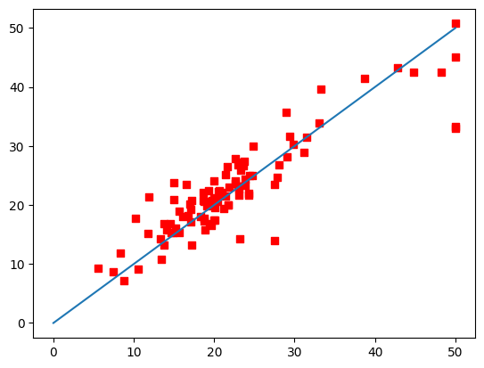
# Visualization of results
# Horizontal axis: values of the teacher data (true prices), vertical axis: predicted values

plt.scatter(y_test, predict, c='r', marker='s') # scatter plot with red square markers.
plt.plot([0,50],[0,50]) # Show a line y=x
plt.show()
[ ]: